Essay 17. Snakes Are Long, Turtles Have Shells: A Reptilian Perspective On Evolvability and Developmental Bias

Three distantly related species of lizard (two Skinks and a Pygopodid) with varying degrees of limblessness. Top Left: Anomalopus verrauxii, Three-Clawed Worm Skink (one-clawed hindlimb, three-clawed forelimb). Top Right: Lerista punctatovittata, Eastern Robust Slider (one clawed forelimb, two-clawed hindlimb). Bottom: Lialis burtonis, Burton’s Legless Lizard (forlimbs absent, hindlimb reduced to scaly flap).

“Ontogeny recapitulates phylogeny.” – Ernst Haeckel, 1866

“The world is a thing of utter inordinate complexity and richness and strangeness that is absolutely awesome.” – Douglas Adams, as quoted by Richard Dawkins in his eulogy for Adams, 2001.

Since the late 19th century and the expansion of Darwin’s revolutionary ideas, laid down in the Origin Of Species and heralded by the vanguard of evolutionary theorists throughout the following years (see Thomas Henry Huxley, Ernst Haeckel, Fischer & Wright, J.B.S Haldane, Theodosius Dobzhansky, Ernst Mayr, to name a few 1, 2) our understanding of life’s inner workings has grown rapidly. Like the tiny, gill and tail-bearing, fish-like human embryo, somewhere around the four week mark (3), the idea of adaptation via heritable variation and selection has itself grown and developed into a complex, kicking, screaming, rapidly growing field of evolutionary theory. As we are want to do, we even packaged and named this post-Darwinian view, underpinned by molecular and population genetic theories, as the new “modern-synthesis” of evolutionary thought.

It can be instructive to think of a scientific theory as if it were in fact a growing, developing organism. A small, fertile idea develops, nurtured and protected in darkness, until it’s ready to be released upon the world at large, growing further as it interacts with other ideas and concepts as a fully formed theory of it’s own. This can apply not only to individual thought, but also to the somewhat cloistered sphere of academia, often rather isolated from the larger pool of popular zeitgeist.

Metaphors aside, and however insightful or well founded a new idea might be, we often struggle to overcome our inherent biases. Our ancestral, plain-dwelling ape ancestors had little practical use for evolutionary musings, likely more focused on matters at hand, namely survival; the passing of the seasons, the migratory paths of prey, the time to sow seed, the well-being of the local support community, to be fruitful and multiply. An ability to contemplate the passage of eons and the incremental, accumulative, slow change in processes like geomorphology or evolution, was not an immediate necessity, and thus we are not well suited to such long term thinking, having to rely on numbers and symbols to make a type of sense of it all (4). We are all biased in our conceptions of time and place (5).

Bias has an interesting place in evolutionary theory, not just in our perception of time and change, but also it seems in function. To understand this further, let’s return to the Modern Evolutionary Synthesis. Like any young theory, it has room to grow, and “modern”, while perhaps appropriate at any particular time, will almost always seem to be premature in hindsight (see modernism, post-modernism, now post-post-modernism, and more prefixes coming to a store near you!). In fact, growth and development are themselves important parts of a more recent and highly insightful branch of evolutionary research; that of evolutionary developmental biology, or “evo-devo”, an intriguing addition to modern, neo-Darwinian thought, part of the so-called Extended Evolutionary Synthesis which many biologists are recently taking up (1, 6, 7). Evo-devo focuses on how evolution changes developmental patterns in organisms. Such considerations are important, for varying genotypes can only be selected by evolution through expressed phenotypes, and phenotypes are produced from genotypes by the processes of cellular development. Through evo-devo studies, mapping the path from genes to organisms, we can further underpin the mechanisms behind phenotypes and their evolutionary origins, firmly tying genotypic to phenotyic variation via the tools of development. Where does bias enter into the story?

One definition of bias, from the Cambridge English Dictionary, is as follows; the action of supporting or opposing a particular person or thing in an unfair way, because of allowing personal opinions to influence judgment. This very personal, rather teleological example nonetheless can be applied to the downright unemotional theory of evolution and development through a phenomenon called “developmental bias”. Put simply, the processes of cellular development can support or oppose certain phenotypic variants, and this can in turn effect evolutionary dynamics (6, 8, 9). Certain phenotypes may be more or less common or successful, not only due to the genetic mutations underlying them, but also the mechanistic biases inherently involved in developing a whole, complex, living organism from a single celled zygote.

One might, with a stretch imagination, picture the following; pick any species you like and the current, standing variation within it’s population. Imagine all the possible variation in form that it’s genes are capable of producing as a fictional, three-dimensional space (okay, multi-dimensional, depending on your level of maths education or current psychadelic dose), for example, one axis, lets say upward, may feature increasingly tall individuals, another increasingly patterned, and so on, containing all possible variants of phenotype. No need to imagine them all as that’s impossible, all we need is a vague picture the varying phenotypes stretching endlessly in off on different axis. We might even give this imaginary multi-dimensional world a name; phenotypic space (1, 7, 8, 9). Depending on the biases in development and gene regulatory networks, and also the forces of selection, pockets of this space could be more or less difficult for a species to access. Could, as species change over time, their access to different parts of their potential phenotypic space also evolve? (7)

Let’s explore with an example in reptiles; the turtle shell. Of all the reptiles, only the Chelonians (Turtles, Tortoises, & Terrapins) bear a hard, protective outer shell (6). This involves a rather drastic re-arrangement of the skeletal plan. In the majority of vertebrates, the shoulder-girdle sits outside the rib-cage. In Chelonians, the ribs have migrated to the outside to support the shell, resulting in a shoulder-girdle that now sits within the rib-cage. This bizarre re-arrangement allows for the turtle to carry the heavy shell, an amazingly useful defensive adaptation which has allowed the turtle lineage to successfully diversify and survive through the ages.

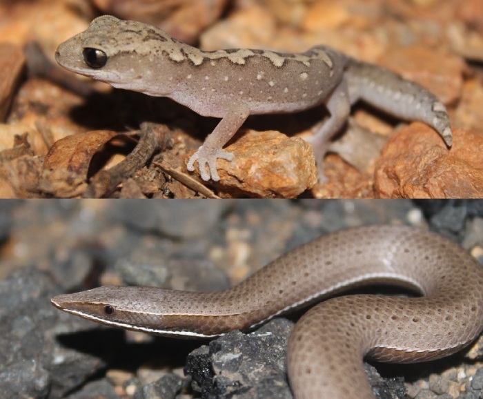
If the turtle’s defensive shell is so darn useful, why then did so few other reptiles evolve a hard shell? There are plenty of independently-evolved shelled invertebrates, from the hard calcium-heavy shells of molluscs and gastropods to varied forms of the exoskeleton in arthropods (6). Shells just don’t seem to be in the reptile’s favoured category of potential shapes. Rather, reptiles lean towards to the lean and long, with elongate body-forms arising independently multiple times, perhaps as many as fifty (6, 9). Consider the legless-lizards of the family Pygopodidae, actually a family of gecko which appear completely limbless, retaining only vestigial leg and hip bones covered by a flap of scale, all that remains of the now degenerate leg (10, 11). Other families of lizard have also evolved towards the long and legless, such as the slider-skink genus Lerista, small burrowing lizards common throughout Australia’s arid areas, all in various stages of leg-loss. Some still have all four legs, albeit often tiny and in stages of reduced digit number, with names like King’s Three Toed Slider (Lerisa kingi) or the Nubbined Fine-Lined Slider (Lerista colliveri). Some have lost their front toes completely, others have no front legs but still have rear legs, often with reduced digits, and a few are entirely limbless (10, 11, 12).

Were we to view this scenario from a purely traditional evolutionary perspective, one might be led to assume that natural selection favours the elongate over the shelled reptile in general, rapidly selecting against those that get all shell-y. This seems unlikely; the defensive nature of the shell has clearly been useful for turtles as it’s a rather ancient body plan (13) that hasn’t gone extinct along with some unfortunate crew of failed ancestors. Rather, they’ve radiated and diverged into multiple forms on land, freshwater, and ocean, clearly demonstrating the evolutionary utility of the shell through a myriad of successful ancestors (10). Selection alone doesn’t suffice to explain the shell’s rarity among reptiles.

The evo-devo perspective introduces developmental bias as a potential solution. Elongate body forms are simpler, with perhaps many potential developmental pathways leading to elongation, easier to access in phenotypic space. A massive, physiological re-design such as shell formation involves a series complex developmental changes to the body plan, perhaps more finite in it’s possible developmental and genetic arrangement (6, 7, 9). Elongation is simpler than shell development and all that comes along with it, thus development and evolution is biased against shelled vertebrates. This part of phenotypic space has been annexed.

Developmental bias has typically been thought of in terms of constraint; shelled animals are constrained to being shelled and so on (1, 6). This rather limiting view has more recently been expanded on as biologists realized that bias is not always negative. One can quite easily turn the above example of elongation on it’s head and say that reptile evolution is positively biased towards elongation (6).

So, there is both negative and positive bias in development, and also in the range of variation that can be produced by an organism. There’s only so many successful ways to develop the turtle shell (6, 9, 13), whereas elongation can happen in a variety of ways; snakes have elongated the trunk of the body and have a rather short tail, whereas most legless lizards (in fact many lizards in general) are about fifty-percent tail (10, 11). We’ve discussed the idea of negative bias, via developmental constraint on phenotypes, and it is quite straightforward, however it’s completeness and explanatory power in real-world evolutionary dynamics had been questioned. More recently, the concept of positive bias (also called developmental drive) has been expanded on (1, 6), showing it can conceptually encompass negative constraint as well as adaptive evolution and the production of novelty.

Here we must first introduce an evo-devo term that includes the idea of positive developmental bias, and also hits the ear nicely, being rather explanatory in it’s very composition; evolvability. Put simply, it is the ability of organisms to generate heritable phenotypic variation (1, 7, 9). This involves not only the heritable genotype but also the processes of development which produces the genotype, processes which may be constrained or promoted. As noted before, certain body systems are more likely (elongation) to evolve than others (shells), and these positively biased systems may in themselves be biased to produce more variation. Birds, for instance, have a highly evolvable body plan and have radiated into maybe more than 19,000 species worldwide into a huge variety of forms (14). Conversely, their closest relatives within the reptilian clade Archosauria, namely the Crocodylians (crocodiles, alligators, and gharials), is comprised of only some twenty-three relatively similar species (15). Developmental processes, evolutionary history, and genetic architecture of birds is evidently much more “evolvable”.

What makes one system more evolvable than another? Our prior example of elongation and shell might suggest that simplicity leads to evolvability, with the complex body plan being limiting for turtles (6). This need not always be; birds are after all rather complex! In fact complexity can, and in biological systems often does, beget complexity (7). This is true for both micro-evolution, the adaptive evolution of form within species, and macro-evolution, the evolution of new species. In micro-evolutionary terms, new adaptations present an opportunity for further change, such as further modification of scales or feathers, stacking change upon consecutive change. On the molecular level, this may be achieved by new point mutations and the opportunities that arise with the associated phenotypic changes, or sometimes by chromosomal events such as gene duplication, providing a second copy of a certain gene which, being redundant, has freedom to mutate and vary. As for macro-evolution, there are boundless examples of species radiations (16, 17, 18), where genetic architecture and novel adaptations may produce a lineage with great potential to split and produce more lineages.

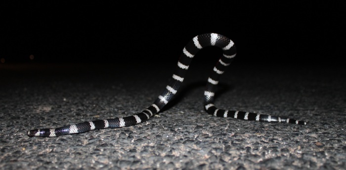
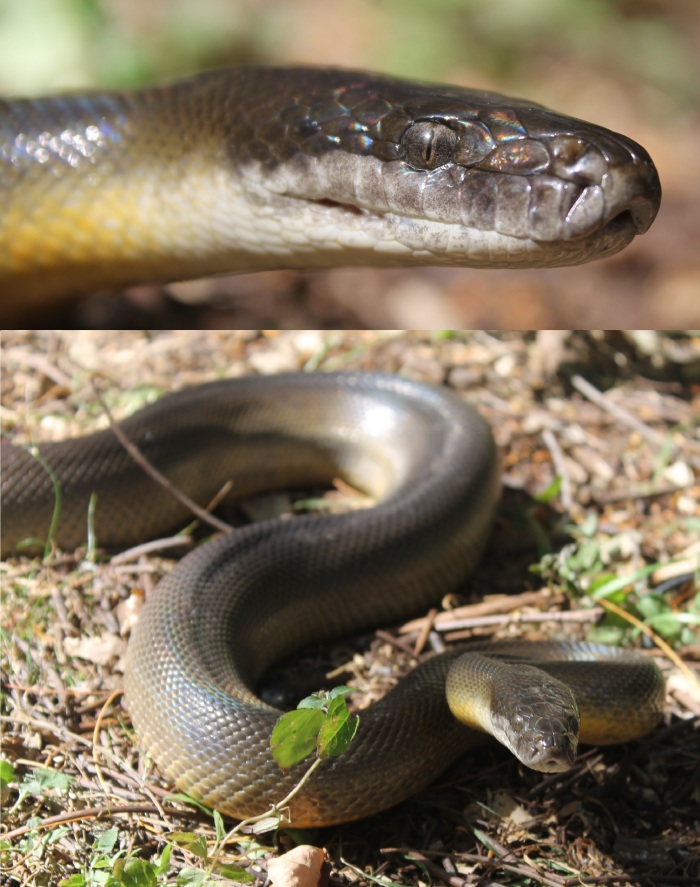
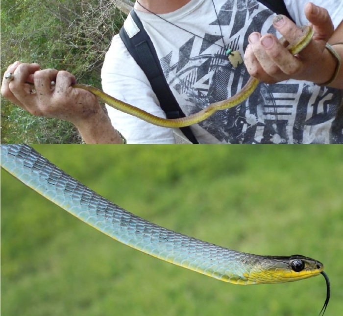
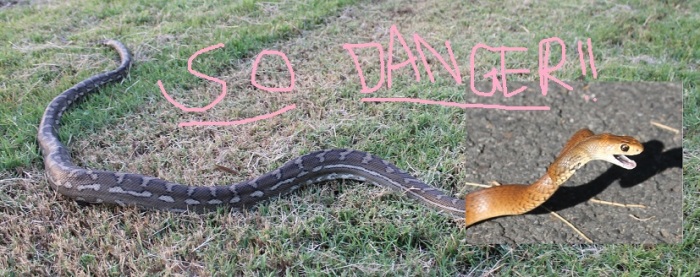
Australian front-fanged snakes of the Elapidae family experienced such a species radiation in relatively recent evolutionary history, the majority arising in the last ten million years (17, 18). As such, the Australian Elapids appear to be highly evolvable in both macro- and micro-evolutionary senses, not only producing a great many species but a wide diversity of body plans, including the strikingly banded and blunt burrowing Simoselaps genus, the incredibly chunky and viper-like Death Adders (Genus Acanthophis), the slender, light-weight Whipsnakes (Genus Demansia), and several long, robust, powerful groups such Taipans (Genus Oxyuranus), Brownsnakes (Genus Pseudonaja), and Blacksnakes (Pseudechis), to name just a few (10, 11, 17). Life-histories vary greatly; there are nocturnal frog specialists, burrowing lizard hunters, large and active mammal predators, ambush strikers, even various aquatically adapted or arboreal species (11). To explore how Elapids came to possess this highly evolvable and adaptive nature, we must delve into their past.

Perhaps as recently as 12 million years ago, the ancestral Australian elapid, likely similar to the south-east Asian coral snakes, arrived in northwest Australia (16, 17, 18). Let’s consider the first arriving corals from south-east Asia as they colonise and expand their numbers somewhere in the northwest corner. With hindsight, we can say that this population will, over time, produce an incredible species radiation as they spread across the country into new habitat pockets and novel adaptive environments. The ancestral population of arriving corals must have held some serious evolutionary potential, unleashed on a continent thus far devoid of modern snakes.

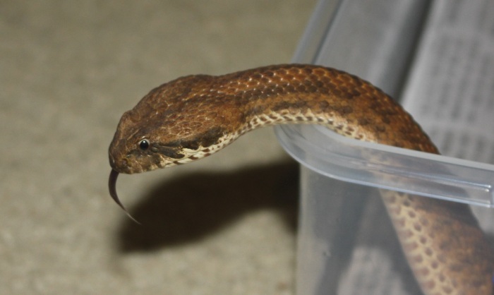
While we can no longer examine these ancestral coral populations, we can make some basic assumptions based on recent observations. Molecular genetic studies of Australian elapids have been rather informative. As expected from their hypothetical origins in south-east Asia, the Melanesian Micropechis genus is found to be the sister group to the Australian elapids and their immediate relatives, namely the basal south-east Asian genera Aspidomorphus and Toxicocalamus (17). Certain morphological characters, such as partial retention of the choanal process of the palatine bone, are common among the south-east Asian forms, but are rare among Australian forms (eg. choanal process only found in the basal lineage Cacophis, the Crowned Snakes). We might assume from this that during their radiation, feeding specialization was a huge adaptive pressure (as seen in other reptiles such as lizards and crocodiles), with new prey types requiring new hunting tools including scent detection, changes in head shape, even the evolution of new venom cocktails (18, 19). As new niches were colonized and, by some means or other, reproductively isolated from one another, adaptation and speciation continued across the continent.

One secret to the success and evolvability of elapids may lie in their history. The sub-order Serpentes is an ancient lineage, speaking volumes to the evolutionary utility of elongation. However, modern snakes are a true marvel of evolution (before we go on, we must again acknowledge the shifting landscape of taxonomy, undoubtedly changing the following “facts” in short-order, but we persevere as best we can). Within the Serpentes, there are two infraorders; Scolecophidia, the ancient, all-burrowing thread and blind-snakes, and the Alethinophidia, or “true snakes”. The majority of basal Alethinophidians can be grouped within the superfamilies Amerophidia and Uropeltoidea, leaving the superfamilies of Pythonoidea, Booidea, and Colubroidea (16). These latter three were previously grouped within the clade Macrostomata, meaning “large opening”, however molecular evidence indicates that their unifying morphological characters might be independently evolved, or at least evolved in a very ancient ancestor prior to separation and divergence (20). Nonetheless, these three genera possess in their skull a hinged supratemporal bone, increasing the flexibility of the skull (19, 20). It is this hinged supratemporal, along with associated changes in jawbone length and more, that allow for the seemingly unnatural ability of many modern snakes to swallow objects vastly larger than their own head.

Following the evolution of the “hinged-jaw” in the Macrostomata, a possibly defunct classification but a good descriptor nonetheless (19, 20), one superfamily within the infraorder Alethinophidia became hugely successful, namely the Colubroidea. Within this group, the family Colubridae is perhaps the most successful modern snake family, comprised of over 1900 species, more than 50% of all currently know living snakes (21), possessing diversity of head shapes and favoured prey, some with well developed rear fangs and venom systems. Other super diverse families include the Elapidae, Viperidae, and Lamprophiidae, each containing more than two hundred species, with a few others such as the semi- to fully aquatic Homalopsidae containing moderate diversity (interestingly, some Homalopsids have evolved a bizarre diet of soft-shelled mangrove crab legs, tearing limbs off their still living victims like schoolkids showing early signs psychopathy). This vast number of Alethinophidian species seems to suggest a high level of evolvability in those lineages also experiencing significant amounts of skull evolution, perhaps even a connection between the two.

This is a tantalizing idea; that the evolution of a highly evolvable skull shape in snakes led to much of their modern success. Without such adaptive flexibility the evolution of the fang apparatus, especially the retractable fang-on-a-hinge system found in Vipers, might not have happened. Recent work combining geometric morphological methods with phylogenetic and ecological data suggests this may not be the first time that changes in head shape led to a significant evolvability in snakes (19). Reconstructing the cranial morphology of their most recent common ancestor suggested characteristics typical of a fossorial burrower, such as a more cylindrical skull, widening of the parietal region, and a reduced/curved quadrate bone. Taken together, the data suggests that terrestrial lizards at some point took to a more burrowing lifestyle, losing their legs and going through changes in head-shape to become the ancient ancestral snakes, which then returned to a life largely above ground. What they brought with them was a skull, genes, and developmental system that was biased towards rapid evolutionary change. Phenotypic space for the future of snake-skulls was an open meadow.

Alethinophidians took this penchant for skull-fidgetry even further. Quadrate bone shaft elongation and curvature, caudal projection, shortening of the snout, all improved flexibility and gape size (19). It seems only right that venom and it’s associated delivery mechanisms arose to prominence in the highly evolvable post-Alethiophidia snake skull. What comes as a surprise is that the first true adaptive novelty was likely due to a burrowing lifestyle, later abandoned by many, followed by further changes to accommodate bigger prey items. This tinkering with the head-shape eventually led to the first snake fang, a rudimentary, elongated rear tooth around halfway down the jawline as seen in some modern colubrids, now grooved for greater venom delivery from the comparatively rudimentary venom glands. The rear jaw elongated, migrating the fang forward over time, resulting in the fore-fanged Elapids and Vipers (22).

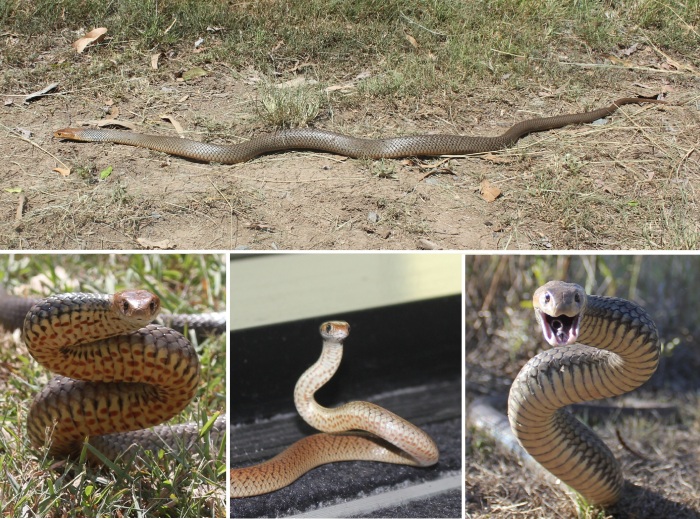
Additionally, with a mass of potential biological interactions, venom genes evolved rapidly, duplicating and diverging into an array of different venom gene families (18). Venom itself is certainly a highly evolvable system, with local prey adaptations found even within species. For instance, South Australian eastern brown snakes are far more toxic to reptiles, their likely prey given the more arid environment compared to the verdant east coast where the same species is much more dangerous to mammalian prey (23). Whether binding to nerve receptors to disrupt signals to the circulatory or respiratory system, interfering with intricate blood clotting cascade, or other physiological effects, venoms have a direct molecular level interaction with their prey. These finely tuned interactions are likely under high selective pressure, but variation in a redundant duplicate copy of a venom gene might well lead to advancements in toxicity.

Venoms, born of a highly evolvable system, must by their nature be rapidly changing, as their prey population will likely develop a defense or immunity, often kicking off an arms race between predator and prey, further accelerating the rate of evolutionary change. Such radical changes in body plans of living organisms may have had a greater influence on evolution than previously appreciated. As a final thought, consider the dramatic increase in evolvability (in terms of complex forms at least) following one of the critical first major steps in the evolution of complex life, the evolution of multi-cellularity (7). Without it, none of us, from salad to snake to scientists, would come to exist, life remaining confined to tiny world of singled celled micro-organisms.

One hates to close a supposed science essay with such an egregious heaping of abstract conjecture. It is, however, at times necessary to take imaginative leaps and bounds. After all, evolution, evo-devo, and the extended evolutionary synthesis are but growing, developing bodies of thought, only recently finding their way into the light of the world, slowly standing up on still wobbly legs and learning to walk. And kids, with their developing, imaginative minds, learn mighty fast. Such is life.

References

1. Brigandt, I. (2015) From Developmental Constraint to Evolvability: How Concepts Figure in Explanation and Disciplinary Identity. In Alan C. Love (ed.), Conceptual Change in Biology: Scientific and Philosophical Perspectives on Evolution and Development. Dordrecht: Springer. pp. 305-325

2. Charlesworth, B. (2017) Haldane and modern evolutionary genetics. Journal of Genetics. 96, 5: 773–782 https://doi.org/10.1007/s12041-017-0833-4

3. Graham, A., & Richardson, J. (2012) Developmental and evolutionary origins of the pharyngeal apparatus. EvoDevo. 3: 24. doi: 10.1186/2041-9139-3-24

4. Knoll, A.H., & Nowak, M.A. (2017) The timetable of evolution. Science Advances. 3: 5, e1603076 DOI: 10.1126/sciadv.1603076

5. Haselton, M. G., Nettle, D., & Andrews, P. W. (2005). The evolution of cognitive bias. In D. M. Buss (Ed.), Handbook of Evoluionary Psychology {pp. 724-746). Hoboken, NJ: Wiley.

6. Arthur, W. (2006) Evolutionary developmental biology: developmental bias and constraint. Encyclopedia of Life Sciences. doi:10.1038/npg.els.0004214.

7. Pigliucci, M. (2008) Is evolvability evolvable? Nat Rev Genet. 9(1):75-82. doi: 10.1038/nrg2278.

8. Psujek, S.,& Beer, R.D. (2008) Developmental bias in evolution: evolutionary accessibility of phenotypes in a model evo-devo system. Evol. Dev. 10: 375–390. https://doi.org/10.1111/ j.1525-142X.2008.00245.x

9. Uller, T., Moczek, A.P., Watson, R.A., Brakefield, P.M., Laland, K.N. (2018) Developmental Bias and Evolution: A Regulatory Network Perspective. 209(4):949-966. doi:10.1534/genetics.118.300995.

10. Cogger, H.G. (2014) Reptiles and Amphibians of Australia. 7^th Ed. Reed Books, Sydney, NSW

11. Shine, R. (1991) Australian Snakes – A Natural History. Reed Books, Balgowlah, NSW

12. Skinner, A., & Lee, M.S.Y. (2009). Body form evolution in the scincid lizard clade Lerista and the mode of macroevolutionary transitions. Evolutionary Biology. 36 (3): 292–300. doi:10.1007/s11692-009-9064-9.

13. Brinkman, D., Rabi, M., Zhao, L. (2017) Lower Cretaceous fossils from China shed light on the ancestral body plan of crown softshell turtles (Trionychidae, Cryptodira). Sci Rep. 7(1):6719. doi: 10.1038/s41598-017-04101-0.

14. Barrowclough, G.F., Cracraft, J., Klicka, J., Zink, R.M. (2016) How Many Kinds of Birds Are There and Why Does It Matter? PLoS One. 11(11): e0166307. doi: 10.1371/journal.pone.0166307

15. King, F.W., & Burke, R.L. (1989) Crocodilian, Tuatara and Turtle Species of the World: A Taxonomic Reference. Wash. D.C.: Assoc. Syst. Collections

16. Reynolds, R.G., Niemiller, M.L., Revell, L.J. (2014) Toward a Tree-of-Life for the boas and pythons: Multilocus species-level phylogeny with unprecedented taxon sampling. Molecular Phylogenetics and Evolution. 71: 201–213

17. Sanders, K.L., Lee, M.S., Leys, R., Foster, R., Keogh, J.S. (2008) Molecular phylogeny and divergence dates for Australasian elapids and sea snakes (hydrophiinae): Evidence from seven genes for rapid evolutionary radiations. Journal of Evolutionary Biology. 21(3):682-95

18. Jackson, T.N.W., Koludarov, I., Ali, S.A., Dobson, J., Zdenek, C.N., Dashevsky, D., Op den Brouw, B., Masci, P.P, Nouwens, A., Josh, P., Goldenberg, J., Cipriani, V., Hay, C., Hendrikx, I., Dunstan, N., Allen, L., Fry, B.G. (2016) Rapid Radiations and the Race to Redundancy: An Investigation of the Evolution of Australian Elapid Snake Venoms. Toxins (Basel). 8(11): 309. doi: 10.3390/toxins8110309

19. Da Silva, F.O., Fabre, A.C., Savriama, Y., Ollonen, J., Mahlow, K., Herrel, A., Müller, J., Di-Poï, N. (2018) The ecological origins of snakes as revealed by skull evolution. Nat Commun. 25;9(1):376. doi: 10.1038/s41467-017-02788-3.

20. Streicher, J.W., & Ruane, S. (2018) Phylogenomics of Snakes. In: eLS. John Wiley & Sons Ltd, Chichester. http://www.els.net [doi: 10.1002/9780470015902.a0027476]

21. “Colubridae” at The Reptile Database. EMBL. Accessed on 8/08/2018.

22. Vonk, F.J., Admiraal, J.F., Jackson, K., Reshef, R., de Bakker, M.A.G., Vanderschoot, K., van den Berge, I., van Atten, M., Burgerhout, E., Beck, A., Mirtschin, P.J., Kochva, E., Witte, F., Fry, B.G., Woods, A.E., Richardson, M.K. (2008) Evolutionary origin and development of snake fangs. Nature. 454, 630–633.

23. Skejić, J., & Hodgson, W.C. (2013) Population Divergence in Venom Bioactivities of Elapid Snake Pseudonaja textilis: Role of Procoagulant Proteins in Rapid Rodent Prey Incapacitation. PLoS ONE 8(5): e63988. doi:10.1371/journal.pone.0063988

Essay 16. A Band of Banded Bandy-Bandy: Evolutionary Musings On A Newly Described Species of Bandy-Bandy Snake

Fig 1. Common Bandy-Bandy (Vermicella annulata) from south-east Queensland presenting the bizarre “hoop-snake” defensive display.

“Evolutionary ‘sequences’ are not rungs on a ladder, but our retrospective reconstruction of a circuitous path running like a labyrinth, branch to branch, from the base of the bush to a lineage now surviving at its top. ” – Stephen Jay Gould, Ever Since Darwin, 1977

“There is no better high than discovery.” – E.O. Wilson

 

With over a thousand species of reptile in Australia described since the arrival of British colonialists in 1788 one might suspect the task of collating an inventory of the country’s snakes, lizards, turtles, and crocodiles would already be complete (1,2). Not so, and when considering the territory, it’s hardly surprising. Australia has the highest reptile diversity of anywhere in the word, not just in number but in uniqueness, some 93% being endemic to the country (3). Despite the tireless effort of herpetologists, a couple of centuries is simply too short a time to catalog the entirety over such a large area, often remote, hazardous, and difficult to survey.

While we may lament the incompleteness of our knowledge, particularly for conservation and management which require solid ecological information, the opportunity for discovery also awaits. And so, every now and again, we’re gifted with a new species. I, of course, say “new” only in terms of our understanding, these species having been in existence since far before the arrival of the first hominids, going about their scaly days with, I presume, little concern for the state of reptile taxonomy. Nonetheless, how these discoveries are made is often fascinating, and the past month has given us several fantastic examples of how scientists add new creatures to our sphere of knowledge. Let us examine one, the discovery of a fine new species of black-white banded snake, Vermicella parscauda, from the Vermicella genus all known as Bandy-Bandy (4).

Like many new species descriptions, hints of their existence, such as suspicion about museum specimens, might have eventually led to a more concerted effort and a definitive conclusion (see this great blog from Australian Museum’s Dr Glenn Shea, 5). Not so in this case, as new specimens can also appear fortuitously. In 2014, while returning from sea-snake field surveys near the town of Weipa in northern Queensland, a team of herpetologists including Professor Bryan Fry from the University of Queensland and Freek Vonk from the Naturalis Museum found a single Bandy-Bandy on a seaside concrete wharf. Initial examination revealed it had some atypical characteristics for the species known from the area (4). Such findings are, for reptile folk, well worth following up.

This is an incredible chance discovery, the snake being accidentally transplanted in mined bauxite rock, left on the wharf awaiting a transport ship. A second and third specimen were found by ecologist Lauren Dibben, dead on the road close to the bauxite mine and alive in it’s nearby natural habitats around Weipa (4). She also provided several past photos of likely suspect Bandy-Bandy, and identified two specimens of the new snake occurring in museum collections. Herpetologist Chantelle Derez identified a further two specimens in museum samples. The evidence for a new species was mounting, but needed confirmation and consolidation with more data.

Before we go on too much further, a question arises; how do scientists name species? This in itself is a complex topic, and having being covered elsewhere (See Essay 13 in this series, 6, or this description of on a new Death Adder species from a few years ago, 7), we will here only cover some essentials. In the field of taxonomy, species are defined or “delinneated” based on a group of variable characteristics, shared more commonly within the species group dataset than between different species datasets. These differences can be physical traits, morphological characters such as size and shape of various body parts, colour patterns, and so on. They can also be molecular, either varying chromosome numbers or structure, protein types and sizes, or the more modern methods involving variation in DNA or RNA sequences. Depending on the data, statistical methods are used to examine how variation is partitioned within or between putative and known species, and how species relationships are diagramatically represented in phylogenetic trees. The field of systematics deals with the evolutionary relationships between these separate species. Such data and new binomial species names (categorizing life into sequentially smaller ranks of Kingdom, Phylum, Class, Order, Family, down to the Genus and Species, as in our own binomial Homo sapiens, of genus “Homo”, and species “sapiens”) can be submitted to the The International Commission of Zoological Nomenclature (ICZN), under a set of formal conventions and naming rules, to be assessed for inclusion as an official new species.

Such procedures, however, are not without their difficulties or controversies. The ICZN code and the rules by which naming occurs can be somewhat arbitrary, allowing for dubious submission, duplicates, and other errors (8, 9). Different source data (e.g. different sets of physical traits, or morphological vs molecular datasets in general), and differences in statistical analyses (e.g. the varying weighting of one character trait over another, or choosing a model of sequence evolution for DNA data) can lead to different results for the same sampled individuals (6, 10, 11). Increasingly, methodological advances in both morphological and molecular taxonomy are improving the situation, however while the general consensus seems to be to flank the species question from both sides, modern molecular methods and their ever improving technology seem to be leading the charge (4, 6, 12, 13).

Returning to V. parscauda, the task of morphological and molecular examination (not to mention the all important manuscript preparation) fell largely upon Chantelle Derez, herpetologist and student of Professor Fry at UQ (4). This involved taking snout-vent lengths, numbers of body/tail bands, and collecting various head, body, and scale measurements from 35 museum specimens of V. intermedia (n = 13), V. multifasciata (n = 6), V. snelli (n = 10) and V. vermiformis (n = 6), using measurement methods and morphological data from Keogh & Smith’s 1996 study of over 400Vermicella specimens (14). The combined datasets were used for Analysis of Variance tests for morphological differences between species groups. On the molecular front, tissue samples from 23 samples were DNA sequenced for the mitochondrial genes 16S (small sub-unit ribosomal RNA gene) and ND4 (NADH-ubiquinone oxidoreductase chain 4 gene), among the most commonly used in snakes studies (4, 7, 13). Additional Vermicella DNA sequences from the online repository GenBank were included in the final phylogenetic analyses, conducting both maximum likelihood and Bayesian Inference analyses, and assessing evolutionary differentiation from DNA sequence variation proportions.

From such a comprehensive overview, species can not only can be delineated from their nearest relatives, but also provide fascinating evolutionary and biogeographic insight, nested within a greater, group context. For example, the data indicates that V. parscauda is clearly a separate species. Genetic variation within the species came to 0.002, while differentiation from its closest relatives, V. multifasciata and V. intermedia, is three-fold higher (0.038 and 0.039 respectively) (4). While the phylogenetic tree also supported the monophyly of the new species, neither the tree nor genetic differentiation suggested significant variance between V. intermedia and V. multifasciata, species recently split out and named based on morphology alone (14). In fact, the tree supported the two being within a single closely related group. Further work may show that these two are in fact a single species, populations perhaps isolated by some change in their ancestral habitats in the monsoonal north.

The Bandy-Bandy genus, Vermicella, are visually stunning, all possessing various numbers of distinct white or pale bands on a black or dark brown body, as their name suggests. In fact, these incredible snakes will often readily display their banded-ness, raising high one or more hoop-like arks of the body as a visual threat response, thus their moniker, the Hoop-Snake (see Fig. 1). When on the move, the black and white banding can seriously confuse the eye, somewhat like the staccato effect of a nightclub strobe-light, disappearing like a gray ghost-snake into the leaf litter. Five species were known to occur (V. annulata, V. intermedia, V. multifasciata, V. snelli, and V. vermiformis), and aside from V. snelli in the Pilbara region, all inhabit non-overlapping distributions across the monsoonal north of Australia, with widespread V. annulata also establishing south along the east coast into Victoria and South Australia, and localized populations of V. vermiformis in central Australia and Arnhem Land (1, 2, 4). Bandy-Bandys are also intriguing examples of several ecological and evolutionary principles, such as niche exploitation, co-adaptation,and homology via convergence or descent, to name a few. The new species, like most recently described and little known critters, is also interesting from a conservation perspective, and we shall examine why in brief.

It is always interesting to investigate the evolutionary origins of such newly discovered species. Where and when did they evolve, and how do they fit into the overall picture of Bandy-Bandy evolution? Before we address this, let’s briefly look at the question more broadly; how do new species arise? While there is still ongoing debate as to what factors influence speciation and rates of lineage diversification, whether, for example, population demographics or environmental variation have a greater influence on the number of species arising over time (15), the general mode of speciation can be summarized as follows; within a population of varying individuals, a small number becomes isolated by some mechanism (discussed below), reproducing among one another but not with the rest of the population pool, over time developing so many differences via adaptive evolution, genetic drift, and mutation, that they can no longer interbreed with their former population. Voila! New species, baby!

OK, so things are perhaps not so straightforward. This glaring oversimplification glosses over many a detail, for example the mechanism of isolation. Allopatric speciation involves populations physically separated by some geographical boundary, parapartic involves individuals entering a new adaptive niche still physically in contact with the source population, peripartic occurs with individuals entering a new niche only partially separated by physical boundaries (essentially a subtype of allopatric speciation), while sympatric speciation, perhaps the most debated of the lot, involves no geographical isolation, only new polymorphisms and phenotypes arising within a population to out-competing or exploiting a niche thus unfilled by its congeners. Further, to grasp the whole evolutionary spectacle, we must appreciate not just isolation mechanisms, but the source material of varying individuals in the population, aka genetics, and quirks of DNA chromosomes such as polyploidy, which we shall unfortunately leave for another time, for the details are as spectacularly fascinating as they are complicated (but read 16 on ploidy and speciation).

Enter the Bandy-Bandy. These snakes are an incredibly well adapted specialist predator (1, 17, 18). How they evolved is somewhat of a mystery yet to be explored, but their natural history is informative. The entire group of snakes live primarily underground, are nocturnal, and feed entirely on other snakes. More specifically, members of the Bandy-Bandy genus (Vermicalla) each feed almost exclusively on several locally co-occurring species of blind snakes, members of the Family Typhlopidae, mostly within the Australio-Papuan genus Anilios, all which live underground and feed on ants, termites, and their eggs or larvae.

The Blindsnakes (Family: Typholpidae) long ago adapted to a life eating ant eggs underground (1, 2, 14). They are small, have smooth, reduced, hardened body and head scales, with an overlapping rostral scale forming a shovel-like snout for burrowing. As their name implies, they are practically blind, with eyes slowly regressed into degenerate pigment spots, still visible through the scales on the top of the head but barely functional and unnecessary in their generally lightless existence. Despite this, they can track an individual ant’s chemical trail accurately (19). They have developed integumentary glands beneath the head scales and cloacal glands which, at least in some species, are used to ward off the ant armies trying to defend their eggs or even other predatory reptiles, and perhaps can even sequester defensive chemicals from their larval ant prey (20). Typhlopidae are an old family, likely of Gondwanan origin, a highly successful one with over 200 species spread throughout the global tropics and sub-tropics.

It seems surprising that such small, difficult food items would be a source of specialization and new species. However, perhaps due to their uniqueness and success, blindsnakes provide a unique predatory niche for whichever species might manage to adapt to exploit them. Many small Elapid snakes are well suited to nocturnal hunting of fossorial and semi-fossorial reptiles like small lizards (1, 21, 22), so making the adaptive leap to blind-snake specialist is perhaps easier than suspected. Even so, the Bandy-Bandy has taken to it’s novel role with aplomb.

While some predators avoid blind snakes (and ants for that matter) or display a taste aversion, perhaps due to the accumulating defensive chemicals picked up from their ant-heavy diet (20), Bandy-Bandys show no such concern. All Vermicella have reduced tooth number and premaxilliary bone (part of the frontal skull), both likely adaptations to their specialized diet (4, 14, 18, 19). They also appear capable of surviving long periods without food, a handy adaptation when one feeds on rarely seen, worm-like, subterranean snakes. Only 1.1% of wild Vermicella annulata were found to contain food items, compared to an average of 20.3% from 10 other Elapid snakes, but when they do feed they seem capable of amazing feats, sometimes consuming blind snakes of near comparable size as themselves, ballooning out with their gargantuan meal (18). They undoubtedly have also well adapted veromonasal receptors tuned into their specific prey items, capable of following a singular ant’s trails back to it’s nest (19). This suite of adaptations is impressive; colouration, behavioural signals, burrowing ability, digestive ability, and more.

The various Bandy-Bandys and their blindsnake prey are excellent examples of homology at either end of the spectrum. Consider, why are all Bandy-Bandys banded? While there’s likely an adaptive reason for banding in the first place, perhaps so-called “flicker-fusion” ghosting effect for instance, the different species of Vermicella didn’t develop their banded-ness in isolation (14, 18). Rather, the ancestral Bandy-Bandy likely passed down the pigment genes for this pattern. These gene variants were retained in the new species despite accumulating variation, particularly in other traits, including those involved in reproductive compatibility, an example of homology by common descent. On the other hand, we might as accurately assume that the plain, non-banded colour of most blind snakes is also a case of common descent. To assume a highly patterned ancestral lineage independently yet faithfully abandoned its banding in over 200 speciation events seems a stretch, while imagining a plain-looking ancestor producing variably plain blindsnakes seems like less of an conceptual struggle.

To contrast, when comparing the bandy-bandy and the blindsnake groups, certain similarities arise; short tails, reduced eyes, smooth scales, and a shovel-like rostral scale on the snout. These are characteristics of animals evolved to a burrowing lifestyle. While the common ancestor of all snakes may have (MAY have, see 23) been fossorial, the Elapids likely arose from the asian coral snakes, a group of terrestrial stem elapids probably arriving in north western Australia and radiating rapidly over some 10 million years (12, 13). The most basal lineages of the Australo-Papuan radiation include the Melanesian Loveridgelaps (a seasnake), Ogmodon (a semi-fossorial Fijian snake), and Salomonelaps (a diurnal forest specialist from the Solomon Islands). The base elapids were probably no longer entirely fossorial, and the similar burrowing adaptations between both Bandy-Bandy and Blind Snakes (shortened tails,…) are thus examples of convergent evolution, where disparate lineages of organisms stumble upon homologous evolutionary solutions to similar selective environments. The same can be said of many features of living organisms, for example, bats and birds; both evolved the capability for flight independently.

Clearly, the Bandy-Bandy was itself rather successful, for the original seems to have been some further radiations into new species, now tallying 6 if we include V. parscauda (4). The new species is itself informative. While it is similar morphologically to the common V. annulata,in having internasal scales, it has comparatively high levels of banding, closer both visually and genetically to V. intermedia and V. multifasciata than others. These highly banded species appear only in the northern monsoonal areas, perhaps implying that the group itself evolved to take advantage of such conditions. Of these monsoon specialists, V. parscauda appears to be the oldest, its lineage rooted closer to the base of the tree, both V. intermedia and V. multifasciata arising from within it. This suggests that V. parscauda was perhaps the first of the highly-banded monsoonal specialist, a new adaptation, while V. intermedia and V. multifasciata both subsequently acquired high banding via descent. On average, V. parscauda posses 70 black and white bands, beat out only by V. multifasciata at an average of 93, making them the second most banded bandy-bandy to ever be banded a bandy-bandy…moving on!

Speaking on their evolution more broadly, the genetic data and the authors generally support “vicariant speciation events”. This is, effectively, allopatric speciation. Let us explore. Due to environmental barriers, like the Great Dividing Range along Australia’s east coast for instance, populations of the ancestral Bandy-Bandy (similar to the stem Vermicella, V. vermiformis and V. snelli), became isolated from one another. A following cooling period, the cold at high altitudes eliminated further gene flow across the range (24; 25). Isolated on the east of the ranges, the population adapted and, after a time, became reproductively incompatible with their former population, forming what we call V. annulata.

It is interesting to consider the similarity between V. intermedia and V. multifasciata in a speciation context. The genetic evidence certainly suggests they may in fact be the same species, perhaps split into semi-isolated populations as the monsoonal tropics became increasingly isolated (4). Despite this fragmenting of the formerly contiguous monsoon habitat, the two species still occupy similar ranges and may co-occur, perhaps even still sharing genes, the isolation thus far seemingly insufficient to incur full reproductive penalties between mating partners. Perhaps these two lineages are in the process of diverging into two species, and perhaps a greater depth of mitochondrial and nuclear data might resolve their relationships. Whatever the case, it is at this stage based on a small sample size and the authors advocate further investigation into the species status of these two. Ironically, in its discovery and study, the new species V. parscauda may relegate the status of V. intermedia back to a synonym of V. multifasciata, the original species they were split out of by Keogh & Smith in 1996 (14), thus the new discovery may nullify an old one, leaving us with, once again, five Bandy-Bandy species. Such is the necessarily fluid and concomitantly stringent nature of taxonomy.

Let us conclude this meditation with a consideration of the new snake itself and what its discovery means for conservation and biodiversity. For any new species, practically by definition, there is little substantial ecological information, and what is known must be gleaned from limited data. What we can say is as follows; only 6 individuals have been recorded, the likely Cape York habitat also home to broad-scale mining (as shown by the first discovery coming from bauxite rock and another dead on the road near the mine site). Being a burrowing animal, soil disturbance may be a paramount threat to the species. We know little of its population size or extent. Given these details, a more comprehansive understanding of it’s ecology and assessment the need for protective listing by the International Union for Conservation of Nature (IUCN) would seemingly not go astray (4).

However, we must be mindful that a listing is only as good as the actions that follow to improve conservation, and species have slipped through the cracks into oblivion even with their species name was hung high on such a registry. In just one disturbing example, we caused the extinction of the Christmas Island pipistrelle (Pipistrellus murrayi), Bramble Cay melomys (Melomys rubicola), and Christmas Island forest skink (Emoia nativitatis) in just five very recent years, between 2009 and 2014, all which were listed as at risk and likely preventable (26). Assessment without action will lead to us merely observing extinctions, which are likely to continue, unless we as a society alter our current undervaluing of nature and species.

To some, this may all sound rather trivial. After all, one more reptile species in a list over a thousand can seem underwhelming, simply adding another of many styles to the catalog. I would argue different. I would suggest that every single one of our species is a unique and fundamental piece of the beauty of existence, something which we bear some responsibility to care for, at the very least for future generations, but also for ourselves. For Australian can never really be the land of nature and wildlife as our national campaigns seem to promote if we don’t, as a culture, celebrate in wonder the phenomenal diversity and individual glory of our precious native species, both old and new.

Finally, a toasting, raucous cheer to the gang of herpetologists, ecologists, geneticists, and others, all who illuminated our natural world further with this discovery, and of course, to Vermicella parscauda itself. May we not fail you in our duty as custodian.

NOTE – Congratulations and many thanks to Chantelle Derez for her time, her generous notes on earlier versions of this essay, and her ongoing work with Australian reptiles. May there be many more discoveries to come!

References:

1. Cogger, H.G. (2014) Reptiles and Amphibians of Australia. 7^th Ed. Reed Books, Sydney, NSW

2. Wilson, S., & Swan, G. (2017) A Complete Guide to Reptiles of Australia. 5^th Ed. New Holland Publishers.

3. Webb, J.K., Harlow, P.S., Pike, D.A. (2015) Australian reptiles and their conservation. In: Stow, A., Maclean, N., Holwell, G.I., (eds.) Austral Ark: the state of wildlife in Australia and New Zealand. Cambridge University Press, Cambridge, UK, pp. 354-381.

4. Derez, C.M., Arbuckle, K., Zhiqiang, R., Xie, B., Yu, H., Dibben, L., Qiong, S., Vonk, F.J., Fry, B.G. (2018) A new species of bandy-bandy (Vermicella: Serpentes: Elapidae) from the Weipa region, Cape York, Australia. Zootaxa, 4446 (1): 1.

5. https://australianmuseum.net.au/blogpost/amri-news/one-up-one-down-and-one-sideways

6. https://snakesonthebrainblog.wordpress.com/2017/07/04/essay-13-taxonomy-trees-and-delimiting-elapid-species-in-the-age-of-molecular-phylogenetics/

7. Maddock, S.T., Ellis, R.J., Doughty, P., Smith, L.A., Wüster, W. (2015) A new species of death adder (Acanthophis: Serpentes: Elapidae) from north-western Australia. Zootaxa. 4007(3):301-26. doi: 10.11646/zootaxa.4007.3.1

8. http://iczn.org/code

9. Kaiser, H., B.I. Crother, C.M.R. Kelly, L. Luiselli, M. O’Shea, H. Ota, P. Passos, W. Schleip & W. Wüster (2013) Best Practices: In the 21st Century, Taxonomic Decisions in Herpetology are Acceptable Only When Supported by a Body of Evidence and Published via Peer-Review. Herpetological Review 44: 8-23.

10. Ocakoğlu, G., Ercan, İ. (2013) Traditional and Modern Morphometrics: Review. Turkiye Klinikleri J Biostat. 5(1):37-41

11. Suárez-Díaz, E., Anaya-Muñoz, V.H. (2008) History, objectivity, and the construction of molecular phylogenies. Stud Hist Philos Biol Biomed Sci. 39(4):451-68.

12. Sanders, K.L., Lee, M.S.Y., Remko, L., Keogh, J.S. (2008) Molecular phylogeny and divergence dates for Australasian elapids and sea snakes (hydrophiinae): Evidence from seven genes for rapid evolutionary radiations. Journal of Evolutionary Biology 21(3):682-95

13. Keogh, J.S., Shine, R. & Donnellan, S. (1998) Phylogenetic relationships of terrestrial Australo-Papuan elapid snakes (subfamily Hydrophiinae) based on cytochrome b and 16S rRNA sequences. Molecular Phylogenetics and Evolution, 10, 67–81

14. Keogh, J.S. & Smith, S.A. (1996) Taxonomy and natural history of the Australian bandy-bandy snakes (Elapidae: Vermicella) with a description of two new species. Journal of Zoology, London, 240, 677–701.

15. Ashman, L.G., Bragg, J.G., Doughty, P., Hutchinson, M.N., Bank, S., Matzke, N.J., Oliver, P., Moritz, C. (2018) Diversification across biomes in a continental lizard radiation. Evolution. doi: 10.1111/evo.13541. [Epub ahead of print]

16. De Storme, N., & Mason, A. (2014) Review: Plant speciation through chromosome instability and ploidy change: Cellular mechanisms, molecular factors and evolutionary relevance. Current Plant Biol., 1:10-33

17. Shine, R., & Webb, J., (1990) Natural history of Australian typhlopid snakes. Journal of Herpetology 24:357-363.

18. Shine, R. (1980) Reproduction, Feeding and Growth in the Australian Burrowing Snake Vermicella annulata. Journal Of Herpetology. 14(1):71-77

19. Greenlees, M.J., Webb, J.K., Shine, R. (2005) Led by the Blind: Bandy-Bandy Snakes Vermicella annulata (Elapidae) Follow Blindsnake Chemical Trails. Copeia. 2005(1):184-187

20. Savitzky, A.H., Mori, A., Hutchinson, D.A., Saporito, R.A., Burghardt, G.M., Lillywhite, H.B., Meinwald, J. (2012) Sequestered defensive toxins in tetrapod vertebrates: principles, patterns, and prospects for future studies. Chemoecology. 22(3):141-158.

21. Lee, M.S.Y., Sanders, K.L., King, B., Palci, A. (2016) Diversification rates and phenotypic evolution in venomous snakes (Elapidae). Royal Society Open Science. 3(1): 150277.

22. Goodyear, S.E., & Pianka, E.R. (2018) Sympatric Ecology of Five Species of Fossorial Snakes (Elapidae) in Western Australia. Journal of Herpetology. 42 (2): 279–285.

23. Da Silva, F.O., Fabre, A.C., Yoland Savriama, Joni Ollonen, Kristin Mahlow, Anthony Herrel, Johannes Müller & Nicolas Di-Poï (2018) The ecological origins of snakes as revealed by skull evolution Nature Communications. 9: 376

24. Bowman, D.M.J.S., Brown, G.K., Braby, M.F., Brown, J.R., Cook, L.G., Crisp, M.D., Ford, F., Haberle, S., Hughes, J., Isagi, Y., Joseph, L., McBride, J., Nelson, G. & Ladiges, P.Y. (2010) Biogeography of the Australian monsoon tropics. Journal of Biogeography, 37, 201–216.

25. Marin, J., Donnellan, S.C., Hedges, S.B., Puillandre, N., Aplin, K.P., Doughty, P., Hutchinson, M.N., Couloux, A. & Vidal, N. (2013) Hidden species diversity of Australian burrowing snakes (Ramphotyphlops). Biological Journal of the Linnean Society, 110, 427–441.

26. Woinarski, J.C.Z., Garnett, S.T. , Legge, S.M., Lindenmayer, D.B. (2017) The contribution of policy, law, management, research, and advocacy failings to the recent extinctions of three Australian vertebrate species. Conservation Biology, 31 1: 13-23

Essay 15. The Trouble With Translocations: Does Snake Relocation Help or Hinder?

Two local snake species from Brisbane, QLD, Australia, both relocated by the author. ABOVE – A non-venomous Carpet Python (Morelia spilota) consuming an urban prey item, in this case a wandering neighbourhood cat. BELOW- A highly venomous Eastern Brown Snake (Pseudonaja textilis) in an office lunchroom, on the kitchen bench in between the toaster and kettle.

“I hate and fear snakes, because if you look into the eyes of any snake you will see that it knows all and more of the mystery of man’s fall, and that it feels all the contempt that the Devil felt when Adam was evicted from Eden.” – Rudyard Kipling, The Return Of Imray.

Kipling, evidently, disliked snakes. Like many of his era and before, perhaps less today (or so one hopes), snakes were seen not only as a dangerous, venomous, marauding villain, but also a portent of evil, the Devil’s own infiltrator lurking in the Garden, one who knows our weaknesses and tempts us into our sinful demise and exile. While certain cultures like Hinduism and Buddhism included powerful, even benevolent serpent gods (such as the Nagas, now the namesake of the Naja genus of cobras), snakes have an almost universally negative perception in western culture. Here in Australia, where some of the World’s most highly venomous snakes are regular backyard visitors, the attitudes are often no different (1). It’s common to hear “A good snake is a dead snake!”, and no small degree of urban legend when discussing these animals, such as the interbreeding of pythons and venomous Brown Snakes to form dangerous “hybrids”, despite these taxa being in separate families (Pythonidae and Elapidae), and therefore, in some senses, as likely as cats and dogs (Felidae and Canidae families respectively) to produce viable offspring (2).

Aside from the confusion of whether to call ensuing hybrid young a “Cog” or “Dat”, this hybrid-Brown Snake myth exemplifies some of the misunderstandings regarding snakes. They are a hugely persecuted but equally ecologically important clade, some adapting better than others to human modified environments (1,3). As such, many snake fanatics find themselves initially falling into and then following a passion for reptiles as a career in research, management, or herpetoculture. For some, such as myself, we wind up in a career involving snake relocation; the safe capture and removal of snakes causing a risk to people, pets, or in the case of rescues, themselves (4). Following a quick health assessment, we then aim to find suitable habitat within their own ecosystem for release, all working under local and federal wildlife and safety legislation.

While a far cry from the more traditional method of dispatch, usually involving some sort of weaponry, I certainly was rather quick to assume that my own actions have had a net positive effect on snake populations and local ecosystems. Here, at the outset of writing and researching this ramble, nearly five years into managing a snake removal service and even longer as a reptile keeper, carer, and general wildlife enthusiast, I still believe fauna translocation can be a useful method for people and ecosystems. But my conviction that what we do is always positive is certainly not as strong. A number of literature reviews on the subject (5, 6, 7) and a plethora of published studies cast further doubt on the suitability of translocation as a management tool. And so, while I am clearly ethically compromised and heavily biased, may I humbly suggest that we still can, and indeed should, discuss the ins and outs of snake translocation in brief, then move on to examine some pros and cons, based on what evidence is available.

In the case of snakes, translocations are often employed to mitigate threats involved in wildlife interactions, often in urban areas (4,8). In my own area of Brisbane, by far the majority of calls are for non-venomous carpet pythons. Looking at some of my own data (from the current financial year, spanning 1^st of July 2017 to 18^th of April 2018), the vast majority of captures are Carpet Pythons (Morelia spilota, N=181), followed by Common Tree Snakes (Dendrelaphis punctulata, N=22), followed closely by Eastern Brown Snakes (Pseudonaja textilis, N=21). After these comes an assortment of minor players; four Yellow-Faced Whip Snakes (Demansia psammophis), three Red-bellied Black Snakes (Pseudechis poriphyriacus), three Brown Tree Snakes (Boiga irregularis), and a few others, for a total of 38 venomous and 206 non-venomous snakes. These non-venomous species are only moved if there’s a genuine threat; if there are pets at risk on the property, if they’re indoors, or if they’re stuck somewhere people need access to (like cars, offices, or work sites). Handling is, ideally, done with an aim to minimise stress where possible and avoid unnecessary agitation.

Moving wildlife is always a troublesome prospect. As ecosystem engineers on a massive scale, finding suitable human habitat is easy almost anywhere in the world. Most other species are locally adapted to their more immediate environments, but so are populations and individuals. While some species have a fantastic spatial memory which they require for movement within their home range (1, 9, 10), others are simply the local variants which survived best given their adaptive advantage, for example, perhaps dark animals living on dark backgrounds survive their first season while lighter variants are picked off by predators (6, 11). Out of any litter, it’s likely that only a few will pass through the selective sieve of time and chance to reach reproductive age, leaving rather well adapted local populations. In translocating animals, the local conditions are hardly likely to be exactly the same at the release site, thus certain local adaptations may no longer be appropriate, or could even become a detriment. The results tend to suggest that relocation, particularly long distances, is generally detrimental to the animal (5, 6, 7).

To what scale we’re interfering with locally adapted snakes is difficult to determine, however there are multiple studies at least attempting to assess the impact, often by radio-tracking translocated individuals. In the USA, relocated timber rattlesnakes (Crolatus horridus) were shown to have a mortality rate of 55% and more erratic daily movements averaging 123.8 meters per day, compared to 11% and 36.9 meters in resident snakes (12). Following translocation, Heiken et al. (13) also found elevated corticosterone and testosterone levels in Pacific Rattlesnakes (C. oreganus) suggesting the procedure can be rather stressful. Relocated Western Diamond-backed Rattlesnakes (C. atrox) also showed three times higher mortality rates then resident rattle snakes (14), and resident Eastern Hognose Snakes (Heterodon platirhinos) also survived three times longer than transplants (15).

Such findings aren’t restricted to reptiles in the United States. In India, King Cobra (Ophiophagus hannah) studies show significant increases in home range size and average daily movement following relocation (16). The white-lipped pit viper (Trimeresurus albolabris) is commonly found in homes and urban areas in South China where they’re relocated to national parks, with some surprising negative consequences (17). After a 3km translocation, individuals took long straight movements but not homing towards any capture point, although certainly exposing them to risks and increased mortality. Furthermore, translocation resulted in a failed, delayed, or extended onset of winter hibernation, a potentially significant mortality factor (18). Translocated female snakes did not reproduce the following season and suffered 80% mortalities, while all males died before the first summer (17).

Here in Australia, several species also show negative responses following translocation. Tiger Snakes (Notechis scutatus) in Victoria were shown to have home ranges six times the size of residents, and make longer movements than residents do (140 vs 64 meters) (19). A recent project by reptile ecologist Ashleigh Wolfe at Western Australia’s Curtin University (20) on Dugites (Pseudonaja affinis), a southwest Australian member of the brownsnake genus common around the city of Perth, showed a troubling result. All four Dugites were killed following relocations over 3km, while residents moved less than 200 meters also showed 50% mortality. Translocated Dugites also had greater activity ranges and travel distances, prior to death of course. It seems that while certain species like carpet pythons seem well suited for urban life (3, 21), larger, venomous species like the Dugite may struggle, perhaps more so when their movements are disturbed.

A range of unrelated taxa appear to show similar responses. Brush-Tailed Possums (Trichosurus vulpecula) in Melbourne, Australia, and White-Tailed Deer (Odocoileus virginianus) Illinois, USA, both also show high mortality rates, and translocation has frequently failed to limit human-wildlife conflicts in Saltwater Crocodiles (Crocodylus porosus), Grey Wolves (Canis lupus), and Brown Bears (Ursus arctos) to name just a few (5, 6, 7). While it’s fascinating reading, the Herculean pile of translocation studies in other species is going nowhere for now, and I fear I’m in danger of laboring the point. Back to snakes.

Translocation, it seems, is at best a temporary solution to an animal’s presence, not so much a measure against further interactions, nor is it ideal for the animal itself. What does all this mean for snake translocations here in Australia? There does, at the very least, appear to be ways to minimise the impact. Various study species, including Eastern Massassaugas (Sisturus catenatus, 18) in Canada, Western (C. oreganus, 22) & Timber Rattle Snakes in the US (C. horridus, 12, 23) through to Dugites in Western Australia (P. affinis), suggests a positive relationship between translocation distance and mortality rate. This makes intuitive sense, with shorter distance translocations less likely to move an animal out of suitable local habitat which it is adapted to, or even keeping an individual within its own home range (12, 22, 23).

Sadly, we must now return to the human-wildlife conflict. Studies have shown that even short distance translocation is hardly an ideal mitigation measure, as many animals, including Tiger snakes, may return to their homes in or near urban areas shortly after release (19, 7, 10). Here we come to an interesting point. I’d like to suggest that not all nuisance or threatening animals are equal. Let us quickly compare our humble Tiger snake from Victoria to a mammalian predator, for example, a Coyote (Canis latrans). No matter how hungry it is, the former does not, unless mistaken by an unfortunately sudden appearance of toes or pinky fingers in front of it’s face, see you as a prey item.

The same cannot be said of a hungry Coyote wandering through the suburbs (24). Here in Australia, our dangerous Elapid snakes generally make every possible effort to flee and avoid humans (1). Also, snakes are often small and have a habit of exploring crevices and caves, leading them to occasionally enter homes via open doors and windows. Moving them back outdoors or off the property, away from pets and people, is often all that’s needed as they’ll generally disappear into cover immediately after release. Moving large, highly intelligent and spatially sensitive predators that return home and see livestock or humans as prey, like bears, wolves or, closer to home, the saltwater crocodile (Crocodylus porosus), is much more challenging (5, 7, 25).

Another consideration is the specific ecology of the snake in question. For instance, while both displayed an increased risk, the mortality rates following translocation were much lower for Tiger snakes (N. scutatus) than for Dugites (P. affinis). In Butler et al. (2005)’s study, discussed earlier, 3 of 8 translocated and 2 of 6 resident tiger snakes died (19). While there are obviously other variables to consider, the aforementioned 100% mortality rate (4 from 4) following 3km translocation for Dugites is striking (20). Could something about this species be putting it at more risk following translocation? For comparison, consider the 1999 Timber Rattlesnake (Crolatus horridus) study (12), with many individuals surviving after being moved between 8 and 172km. Of two individuals moved 172km, creatively named FOX6-92 and FOX1-91, both survived two seasons of tracking, one eventually succumbing to disease, the other surviving the whole study period. I won’t say who survived, you’ll just have to read the paper, but their name started with FOX…moving on!

Different requirements of the species being moved, as well as the characteristics of surrounding habitat, should be considered. For example, generalist feeders might be more likely to find suitable prey in unfamiliar habitats than specialists (7). Perhaps the Tiger snake, a much more generalist predator, is more capable of finding any number of lizards, birds, rodents, frogs, or even carrion, while the Dugite struggles to find new grounds to hunt rodents and lizards (1, 20). Or perhaps, since these studies haven’t been replicated in different areas, the suburbs surrounding Perth where the Dugite study took place are more hostile to snakes in general than the wetland park where the Tiger snake study occurred. Impacts of attaching transmitters aside, a 50% mortality rate even for resident Dugites moved no more than 200 meters (3 out of 6 died) shows just how dangerous the urban landscapes can be for snakes (20). Previous work by Wolfe and Co. found that urban Dugites were in worse condition, generally smaller and less likely to have prey in their stomachs, suggesting the typical response for urban-adapted predators (i.e. exploiting novel food sources) is not the case for this species (26).

This brings up several questions. What exactly is it about Dugites that makes them so vulnerable? Is it something about their life history or something about Perth’s urban environment? If it’s a case of life history, for example being a specialist feeder, what other species share those characteristics and do they correlate in terms of translocation success? Or, if it’s something about Perth’s urban environment, perhaps an abundance of roaming cats, what other cities are suicide for snakes, and why? It might be interesting to examine how several sympatric snake species (#newbandname #SSSS), perhaps Eastern Brown Snakes (P. textilis) and Red-Bellied Black Snakes (Pseudechis poriphyriacus) fare around large, urban centers along the coast, such as Brisbane, Sydney, and Melbourne.

Nevertheless, until all these variables are known, like a snake catcher under a house, we must grope on in the darkness. However, as a snake catcher, I assume we can try to live by a few short rules based on what we know:

1. Try not to move snakes. It’s counter-intuitive, but the best job is one where you’ve educated a frighted caller and not moved anything. You don’t get paid, but that’s life.

2. If you must move an animal, minimize the distance and choose appropriate habitat, taking into account the species’ ecology, in particular, movement patterns and home ranges, if these are known.

Thus, what is appropriate must be decided on a species by species basis. This, again, gets complicated. For example, Eastern Brownsnakes have been shown to have a larger home range than Tiger snakes, as calculated by Minimum Convex Polygon (MCP, 5.8 vs 3.88 hectares), suggesting some Brownsnakes may handle more distant translocations (19, 27). Mortality rates in Dugites suggest otherwise (20). Further, MCPs can vary hugely. Tiger snakes from the New England plateau have much smaller MCPs of 0.77ha (albeit from small sample size, 2 snakes over 6 weeks, Shine, 1979), and MCPs of the large, highly mobile Burmese pythons in the USA Everglades can range between 170 to a massive 8,740 hectares (10, 28). Even within one Australian species, the carpet python (Morelia spilota), a variety of MCPs have been recorded; 17.6ha (21) and 22.5ha (29), while male and female Diamond Pythons (a dark, speckled M. spilota morph from the Sydney region) have MCPs of 52ha and 27ha respectively (30). Red-Bellied Black Snakes also display a wide range of MCPs, from 0.02ha to over 40ha between individuals, and larger in males during breeding season (9). MCPs and home ranges are thus probably better used as guides, and only relied upon if the spatial ecology of the species is well studied.

Unfortunately this is rarely the case. Rarely do we have a good understanding of a snake species’ movement ecology, though there are exceptions, and generalizations are certainly possible; invasive Burmese Pythons clearly move further than Carpet Pythons, which move further than Brown Snakes, which move further than Tiger Snakes. What movement ecology means for survivorship following translocation, I would suppose, depends on the distance to, extent of, and quality of the new habitat, as well as the condition of the animal before and after handling. Ideally, controlling for these factors, translocation can be improved upon, as appears to have been the case over the years with increasing success rates over the last few decades, likely due to improved methodology (6). While hardly ideal, an understanding of each species home range, their ecology, and the local ecosystems at capture and release seems, to me, the best way forward for now. Nonetheless, while it’s not a huge sample size, four from four dead Dugites (20) speaks for the need for more research, and to potential for our well meaning actions, when not examined, to cause more harm than good.

A final thought. What might be the outcome if we abandon snake translocation entirely? While individuals may certainly be at risk, would snake populations be any worse off if we left an educated general public to deal with snakes on their own, without the experience and training required of professional snake handlers? And what viable options other than translocation are available to us? I don’t know the answer to these questions, but it seems that we are, for now, continuing with the less-than-perfect tool of translocations for snake management. More research into its impacts on various species and local ecosystems certainly would not go awry. Let’s stay on our toes.

References:

1. Shine, R (1991) Australian Snakes: A Natural History. Reed Books, Sydney, New South Wales.

2. https://snakesonthebrainblog.wordpress.com/2017/02/19/essay-10-hybridization-and-the-myth-of-python-brownsnake-crossbreeding/

3. Fearn, S., Robinson, B., Sambono, J., Shine R. (2001) Pythons in the pergola: the ecology of ‘nuisance’ carpet pythons (Morelia spilota) from suburban habitats in south-eastern Queensland. Wildlife Research. 28, 573–579

4. Shine, R. & Koenig, J. (2001) Snakes in the garden: an analysis of reptiles ‘‘rescued’’ by community-based wildlife carers. Biological Conservation. 102, 271–283

5. Fischer, J. & Lindenmayer, D.B. (2000) Review: An assessment of the published results of animal relocations. Biological Conservation. 96, 1-11

6. Germano, J.M. & Bishop, P.J. (2008) Review: Suitability of Amphibians and Reptiles for Translocation. Conservation Biology. 23. 1, 7–15

7. Massei, G., Quy, R.J., Gurney, J., Cowan, D.P. (2010) Can translocations be used to mitigate human–wildlife conflicts? Wildlife Research. 37, 428–439

8. Welton, R.E., Liew, D., Braitberg, G. (2017 Incidence of fatal snake bite in Australia: A coronial based retrospective study. Toxicon 131, 11-15

9. Shine, R. (1987) Intraspecific Variation in Thermoregulation, Movements and Habitat Use by Australian Blacksnakes, Pseudechis porphyriacus (Elapidae). Journal of Herpetology. 21. 3, 165-177

10. Hart, K.M, Cherkiss, M.S., Smith, B.J., Mazzotti, F.J., Fujisaki, I., Snow, R.W. (2015) Home range, habitat use, and movement patterns of non-native Burmese pythons in Everglades National Park, Florida, USA. Animal Biotelemetry. 3:8

11. Dubey, S., Zwahlen, V., Mebert, K., Monney, J., Golay, P., Ott, T., Durand, T., Thiery, G., Kaiser, L., Geser, S.N., Ursenbacher, S. (2016) Diversifying selection and color-biased dispersal in the asp viper. BMC Evolutionary Biology. 15,99

12. Reinert, H.K. & Rupert, R.R. Jr. (1999) Impacts of Translocation on Behavior and Survival of Timber Rattlesnakes, Crotalus horridus. Journal of Herpetology. 33. 1, 45-61

13. Heiken, K.H., Brusch, G.A., Gartland, S., Escallón, C., Moore, I.T., Taylor, E.N., (2016) Effects of long distance translocation on corticosterone and testosterone levels in male rattlesnakes. General and Comparative Endocrinology.

14. Nowak, E.M., Hare, T., McNally, J. (2002) Management of ‘nuisance’vipers: Effects of translocation on western diamond-backed rattlesnakes (Crotalus atrox). Biology of the Vipers. Eagle Mountain Publishing: Eagle Mountain, UT, USA. 535–560.

15. Plummer, M.V. & Mills, N.E. (2000). Spatial ecology and survivorship of resident and translocated hognose snakes (Heterodon platirhinos). J. Herpetol. 34, 565-575.

16. Barve, S., Bhaisare, D., Giri, A. (2013)A preliminary study on translocation of “rescued” King Cobras (Ophiophagus hannah). Hamadryad. 36. 2, 80-86

17. Devan-Song, A., Martello, P., Dudgeon, D., Crow, P., Ades, G., Karraker, N.E. (2016) Is long-distance translocation an effective mitigation tool for white-lipped pit vipers (Trimeresurus albolabris) in South China? Biological Conservation. 204, B, 149-468

18. Harvey, D.S., Lentini, A.M., Cedar, K., Weatherhead, P.J. (2013) Moving massasaugas: insights into rattlesnake relocation using Sistrurus c. catenatus. Herpetol. Conserv. Biol. 9, 67–75.

19. Butler, H., Malone, B., Clemann, N., (2005) Activity patterns and habitat preferences of translocated and resident tiger snakes (Notechis scutatus) in a suburban landscape. Wildlife Research. 32, 157–163.

20. Wolfe, A., Fleming, P., Bateman, B. (2018) Impacts of translocation on a large urban-adapted venomous snake. Wildlife Research. (JUST ACCEPTED, 30 March 2018, WR17166)

21. Shine, R. & Fitzgerald, M. (1996) Large snakes in a mosaic rural landscape: the ecology of carpet pythons Morelia spilota (Serpentes: Pythonidae) in coastal eastern Australia. Biological Conservation. 76, 113–22.

22. Brown, J.R., Bishop, C.A., Brooks, R.J. (2009) Effectiveness of short-distance translocation and its effects on western rattlesnakes. J. Wildl. Manag. 73, 419–425.

23. Sealy, J. (1997). Short-distance translocation of timber rattlesnakes in a North Carolina state park, a successful conservation and management program. Sonoran Herpetologist. 10, 94–99.

24. Poessel, S.A., Gese, E.M., Young, J.K. (2017) Landscape and Urban Planning Research paper Environmental factors influencing the occurrence of coyotes and conflicts in urban areas. Landscape and Urban Planning. 157, 259-269

25. Campbell, H.A., Dwyer, R.G., Irwin, T.R., Franklin, C.E. (2013) Home Range Utilisation and Long-Range Movement of Estuarine Crocodiles during the Breeding and Nesting Season. PLoS ONE. 8(5): e62127.

26. Wolfe, A.K., Bateman, P.W., Fleming P.A. (2017) Does urbanization influence the diet of a large snake? Current Zoology. 39, 1-8.

27. Whitaker, P.B. & Shine, R. (2003) A Radiotelemetric study of movements and shelter-site selection by free-ranging brownsnakes (Pseudonaja textilis, Elapidae). Herpetological Monographs. 17. 1, 130-144.

28. Pittman, S.E., Hart, K.M., Cherkiss, M.S., Snow, R.W., Fujisaki, I., Smith, B.J. (2014) Homing of invasive Burmese pythons is South Florida: evidence for map and compass senses in snakes. Biol Lett. 10, 10, 20140040.

29. Pearson, D., Shine, R., Williams, A. (2005) Spatial ecology of a threatened python (Morelia spilota imbricata) and the effects of anthropogenic habitat change. Austral Ecol. 30, 261–74

30. Slip, D.J. & Shine, R. (1988) Habitat use, movements, and activity patterns of free-ranging diamond pythons, Morelia spilota spilota (Serpentes: Boidae): a radiotelemetric study. Aust Wildlife Res. 15, 515–31.

 

 

 

 

 

 

 

 

Essay 14. Snake Skin, Scales, And The Rainbow of Reptile Colouration

Fig.1. The water python (Liasis fuscus), a large, brownish constrictor common in NT floodplains, with some yellow underneath, while lips, and iridescent shine.

“And that… is the resting place of the Rainbow Serpent, and all of the gullies and all of the lagoon itself was about the Rainbow Serpent created, after he had created the universe…”

-Carl McGrady, Aboriginal Education Assistant, 1996. For more, see australianmuseum.net.au/indigenous-australia-spirituality

Walking through the remote landscapes of Australia, particularly the rocky northwest, you may notice among the ancient plants, animals, mountains, waterfalls, and so on, some truly amazing examples of traditional rock art. Depictions of various totem animals, stories and traditions, important cultural events or encounters, and much more, are all found among the old caves and protected rocky overhangs that served as painting sites for one of the oldest known continuous traditional cultures on Earth, arriving here some 65,000 years ago (1, 2). Among these, artworks of the Rainbow Serpent have been dated to some 6,000 years ago, and it’s pervasiveness among Australian aboriginal culture cannot be understated with dozens of names among many different tribes (3). The Rainbow Serpent is a common motif in many language groups, a Dreamtime creator god being who’s tracks carved rivers, lagoons and other landscape features often associated with life-giving water, yet a dangerous force when angered, a rather apt analogy for both snakes and seasonal, monsoonal flooding events.

In nature, the Rainbow Serpent is represented by several species of snake, depending upon which tribal lore your following (3,4). The Western Australian Noogar people likely considered the Wonambi (Wonambi naracoortensis, from the extinct snake family Madtsoiidae) to be one manifestation of the deity, an ancient and unpredictable spirit of the waterhole. In the North Territory, the iridescent, rainbow-like reflection given by pythons of the extant Liasis genus, including the water python (L. fuscus or “Bolokko”, see Fig. 1) are possible living candidates for the origin of the myth, again suggesting a strong connection to water and seasonality (4).

That said, while it is a fascinating creature in it’s own right, the water python is aesthetically a rather plain, brownish snake, aside from a yellowish belly and some variably white facial patterning (4,5,6). While a large proportion of Australian snakes spend some or a whole part of the life as a brownish flash in the grass, many come in a dazzlingly broad range of colours and patterns, often highly camouflaged but highly conspicuous if removed from their associated environment. The deep ochre red and bright yellow banding of the Desert Death Adder (Acanthophis phyrrus) is an ideal pattern for camouflage among the red sand and dry spinifex in the arid centre of the continent, however it would stand out like a gleaming gem among the darker hues of forest floors on the East coast. Here however, the Common Death Adder’s (A. antarcticus) bands of mottled grey, brown, and black make it supremely hard to distinguish from forest rocks and leaf-litter (5,6, see Fig. 2).

Fig.2. Common Death Adder (Acanthophis antarcticus) from South-East Queensland, out on the road (above) and hidden in leaflitter (below).

Such wide variation can even be found within certain species. For example, the strikingly golden Northern Territory forms of the common tree snake (Dendrelaphis punctulata), well suited to long, dry grasses of their northern habitats, would surly be less successful in southern populations thoughout verdant forest all the way along the coast down to Sydney, where colours range from dark, practically black hues of green, through to light blues and various shades in between (5,6, see Fig. 3). The carpet python (Morelia spilota) is another example of within-species variation with a massive range of colour forms, from the red and cream Centralian desert morphs, to the black and yellow Jungle pythons from rainforests in north Queensland’s Atherton Tablelands, and the lichen-like Diamond pythons usually found in dark, well-vegetated forests of south to mid-coastal New South Wales. In their contextual environments, such patterns make these snakes masters of camouflage and stealth, avoiding detection by both predators and prey. Further patterning is used for a variety of purposes such as behavioural signaling, whether colour cues for communication among individuals, or for threat displays like the prominent bright red spots on the underbelly of eastern brownsnakes (Pseudonaja textilis) (5,6,7, see Fig. 4).

Fig.3. Common Tree Snake (Dendrelaphis punctulata) golden northern territory form (above) and  southern blue and olive (below). There are also many other colour forms, some nearly black, some vibrant green.

I suppose we can confidently say there is some method to this madness, some suite of adaptive forces and selective pressures molding the evolution of colour in snakes. One could hardly expect to constantly find such fantastically adapted populations occurring in their ideal habitats by chance alone! How then do these colour patterns evolve? To answer such a question we need to first understand some basics of colour formation in animals, and for this we must begin with the biology of the organ producing colour: the skin. PS you may also want to note the heavy referencing of Betchel (1995)’s book on the subject, and get yourself a copy (8).

Fig.4. Eastern Brown Snake (Pseudonaja textilis) undisturbed in situ (above) and in threat display (Below, Left to right: same individual as above, juvenile indoors, large adult with faint markings)

Animal skin, including our own, is an organ of soft tissue covering the outer surface of vertebrates. In mammals it consists of two tissue layers, the outer ‘epidermis’ providing protection and waterproofing, and the lower dermis providing structure and other support functions (8, 9). The dermis forms an extracellular maxtrix of various elastic fibers such as collagen embedded in a mix of large molecules called proteoglycans and hyaluronans, as well as hair follicles, nerve cells, and blood vessels providing nutrient and waste transport to both skin layers. Above the dermis, beyond a thin layer of fibres called the basement membrane, lies the epidermis, consisting of about 95% keratinocyte cells. Keratinocytes proliferate by simple mitotic cell division in lowest layer of the epidermis, the Stratum germinativum, with daughter cells migrating upwards as they proliferate. As they migrate they differentiate, eventually losing their nuclei and forming junctions with other anucleated keratinocytes. These junctions excrete keratin and lipid molecules to form the outer layer of tough, keratinzed, dead and dying cells known as the stratum corneum, our outer skin, which eventually sheds in small white flakes, often landing gently on the shoulders of various expensive suits and dresses. Among the keratinocytes will be a few Merkel nerve cells & Langerhan immune cells, as well as the odd melanin-pigment-containing melanocyte cells, providing UV-protection and skin colour (9).

Reptile skin is different from mammals in having less defined layers within the epidermis, a thicker, more keratinized & fibrous stratum corneum, relatively fewer skin glands, and complete lack of hair follicles (Betchel, 1995). Each scale is, in fact, a fold of skin composed of all these skin layers, including a tough and durable outer stratum corneum. It is this dead, outer keratin layer that is shed by reptiles, including the eye caps, a few days after a diffusion of lyphatic fluid separates it from the underlying epidermis. Further down, there are three very important types of colour cells embedded within the dermis, collectively called chromatophores. We’ve already met one, the melanocyte in the mammalian epidermis, full of the dark, light-absorbing pigment called melanin. Reptiles also have dark, scattered melanin cells in their epidermis called melanophores, the diffference being melanocytes excrete melanin outside the cell while melanophores generally keep their melanin inside. In reptiles, melanophores are also found in the dermal layer, particularly in regions of darker scale pattern. The distribution of both epidermal and dermal melanophores help produce the black, brown, and various darker patches of pigment in reptiles. Reptiles can also modify the distribution on melanin pigment within their melanophores, but more on that later.

We’ve seen that both mammals and reptiles share melanin pigment in the production of darker skin. What about the vibrant reds, yellows, and more? These are not the product of melanin, although it’s interactions may be very useful in pattern formation and rapid colour change (8). There are two other chromatophores involved in reptile colouration, namely the xanthophores and iridiophores. The xanthophores are bright coloured cells containing a variety of pigments including red/yellow pteridines (synthesized in the xanthophore) and yellow carotenoids (plant based, part of their dietary uptake and stored in xanthophore). The varying concentrations of these pigments produce red, yellow, and their intermediates. Xanthophores are sometimes further split based on their colour, with those heavy in red pteridines and carrotenoids called erythrophores, while simply “xanthophore” is reserved for yellow cells, after the Greek word for yellow, “xanthos”.

This gives us quite a variety! We have varying shades of black, brown, red and yellow, and while you could almost use these colours alone to draw many of our desert reptiles, there’s much more variety to be had. What of the vibrant greens, blues, whites, even purples, sadly missing in us hominds yet often seen in the great rainbow of snake diversity? Enter the third type or chromatophore, called the iridiophore (8). These produce what are called “structural colours”, based on light-rays reflection and scattering off organelles called “reflecting platelets” within the cell. These platelets are variably arranged in oriented stacks and adorned with crystalline deposits of purine molecules, including adenine, hypoxanthine, and guanine (incidentally, the same guanine used by the genetic code, which we denote as “G”). Based on their size, shape, and arrangement, iridiophores variably produce a wide variety of colours including greens and blues, also interacting with other chromatophores in the skin to produce an even greater range of hues, as well as the rainbow-iridescence seen in some species of snakes (see Fig. 1).

In fact, not only do the three cell types (dark melanophores, warm xanthophores, vibrant and varying iridiophores) interact to produce colour & patterning, they also have the same origin, and even bundle into a unit for rapid colour change in animals such as anoles (8). Let’s wind the developmental clock back on, for example, a Tiger Snake (Notechis scutatus), all the way to the embryonic stage. The cell layers (ecto-, meso-, and endoderm) have all folded and begun to differentiate into the skin, musculature, and intestines respectively (and more, but let’s keep it simple). Also produced from an invagination or folding of the ectoderm is the neural tube, with the neural crest forming at the meeting point of the folded ectoderm. Neural crest cells multiply into chromoblasts, the stem cells of chromatophores, capable of differentiating into melanophores, xanathophores, or iridiophores.

These chromoblast migrate out from the neural crest following other developmental chemical signals to locations in the forming dermis. As our embryo develops, the skin darkens into a banded pattern of browns or blacks as melanin is deposited, included in the retinas where they attach to opsin proteins to produce light vision. Along the body, bars of creamy yellow appear between the dark bands, underlain by xanthophores filling up with pteridines initially, then by carotenoids as they’re depsoited from the yolk. All interact with the wavelength-modifying crystal chandeliers within the dermal iridiophores, particularly where greenish hues are produced. Voila! A juvenile tiger snake, complete with dark olive and bright yellow banding and a lighter grey-green head emerges from the egg, readily camouflaged among the grasses and reed beds of it’s marshy surroundings.

What of those reptiles capable of rapid colour change? Here the chromatophores are bundled into an interacting “functional chromatophore unit” (8). The melanophore is known as a dendritic cell, meaning it has protrusion out of the cell like arms with long fingers. The melanophore sits at the base of the chromatophore unit, it’s dendrites running upwards towards the skin surface. On top on the main body of the melanophore sits the iridiophore cell, then the xanthophore stacked on top. Typically, the majority of the meanophore’s melanin-containing ornganelles, called melanosomes, reside at the base of the melanophore, beneath the iridiophore and xanthophore, absorbing what light makes it past. It’s dendrites, however, reach up past both other cells. Thus, triggered by the secretion of Melanocyte Stimulating Hormone from the anterior pituitary gland, a fast movement of all possible melanosomes from the basal body to the upper dendrites blocks a large portion of incoming light to both the xanthophore and iridiophore, coordnated by the cell’s internal microtubule and actin cytoskelelton, and associated transport enzymes (9,10).

This flow of melanin darkens the skin, however with colour being produced by the complex interaction of the three cell types on the visual wavelength of reflected light, simply varying the distribution of melanin can vary colour more than just dimming or brightening. Changes in bloodflow to the skin can further add vibrancy to this already brilliant display in some species, or deliver stimulating hormones to specific b0dy regions, adding flushes of pattern and colour. Indeed, the very rapid colour change seen in chameleons is actually caused by iridiophore placement in the epidermis. Comparing multiple TEM (transmission electron microscopy) images from individual Madagascan panther chameleons (Furcifer pardalis) found that the reflective guanine crystals in S-iridiophores of resting state skin (blue or green colour)are around 30% closer than those from excited state skin (yellow or white) (11). Excitation causes a rapid spreading out of these nano-crystals within the S-iridiophores, causing the corresponding shift from green to yellow/orange very rapidly.

Additionally, reptiles can also have much slower colour change, generally based on the slow accumulation or loss of melanin from melanosomes and skin (4,5,8). These are often seasonal, such as the darkening and lightening of hue in the inland taipan (Oxyuranus microlepidotus) to moderate fluctuating environmental temperature, darkening in winter to absorb more heat and vice versa. Such changes may also occur along with age, like the dilution of juvenile pattern in aging eastern brownsnakes (P. textilis, though many adults remain patterned), the growth of adult patterning in relatively non-patterned juvenile carpet pythons (M. spilota, see Fig. 5) in their first few months after hatching, or the various age phases from deep red/brown and yellow through striking blue, mottled, and eventually, the glorious green of adult green tree pythons (Morelia virdis).

 

Fig.5. Carpet Python (Morelia spilota), brown neonate (above) and full adult colouration (below)

Of course, things don’t always work out so neatly. With such a complicated system of interacting chromatophores, pigments, blood-flow, UV-absorbance, and prone as biological systems are to occasional mutation and environmental perturbations, errors are somewhat expected (8). These aberrations come in a variety of tantalizing flavours, many due to heritable genetic mutations which snake keepers around the world are keen to introduce into their breeding programs. Some aim to produce proven, true-breeding homozygous (or heterozygous intermediate and codominant), bizarrely coloured snakes for the recreational wildlife market (12).

So many of these exist that the names used by industry bred lines have become commonplace, such as the various axanthic, anerythric, or pie-bald lines of ball pythons readily available in the US market (12). Darker hypermelanistic animals are fairly common in the wild, as are lighter hypomelanistic individuals, and both are sought after by breeders. Even more so are albinos, the well known, red-eyed, light coloured individuals producing very little or no melanin whatsoever, considered a universal mutation and found in practically every animal with enough collected samples (8). Albino reptiles are typically light in colour but still produce yellow and reddish hues via xanthophores & iridiophores.

Alternatively, axanthic snakes appear more on the greyscale, a hereditery defect in xanthophore pigment production (but not in dietary carotenoid uptake), lacking the reds to yellows produced by pteridines (8,10). Axanthic snakes lacking red may also be referred to as anerythristic, lacking the red-heavy xanthophores referred to as erythorphores by some, but this terminology and the associated phenotypes are highly variable. Leucism is an even greater extent of pigment aberration resulting in pure white snakes with regular black eyes (sometimes blue but never the amelanistic red-eye of albinos), involving loss all three chromatophores (no melaophores or xanthophores, few functional iridiophores), however the loss of function is likely due to the skin itself failing to support chromatophore function within the dermis. Those pigments deposited elsewhere such as the retinas are fine.

The function and mode of inheritance for many of these aberrations can be variable, even within a species. Even wild population may contain mutations at multiple loci leading to the same outward appearance (8). Albinism, for instance, is an error in the process of melanosynthesis, by which the amino acid tyrosine is converted into melanin. This involves two oxidation steps, first turning tyrosine into DOPA (dihydroxyphenylalanine) which in turn is oxidized to dopaquinone. These oxidation steps require the catalytic enzyme tyrosinase, after which dopaquinone is finally turned into melanin. We’re we to remove tyrosinase, the oxidation reactions would not occur to produce DOPA or dopaquinone, thus no melanin synthesis. This ‘tyrosinase-negative’ albinism is the most commonly known form, usually a recessive mutation at the gene responsible for tyrosinase production, known in humans as TYR, with albinism occurring due to mutations in about 1:20,000 people (13).

Tyrosinase-positive albinism is the second most frequent form, with functional tyrosinase production in melansomes, however some mechanism fails to transport the necessary tyrosine amino acid to the melanosome for the reaction to begin (8). Despite having both tyrosine and tyrosinase, these individuals look pretty much exactly like tyrosinase-negative albinos, although some tiny amount melanosynthesis may occur throughout the animals lifetime if any tyrosine makes its way to the waiting, functional melanosome. Both types of albinism may occur via mutations at a number of sites, either different loci on the long TYR gene in tyrosine-negative, or via various mechanisms to interfere with tyrosine transport to the melanosome in tyrosine-positive albinism.

With so many possible errors, its little wonder that snake populations, even in the wild where selection pressure is constantly chipping away at such errors, have an estimated albinism rate of between 1:10,000 to 1:30,000 (8). Various brilliantly coloured mutant populations are known to occur, such as the albino Japanese ratsnakes (Elaphe climacophora) found around the city of Iwakuni, hereditary piebaldism in corn snakes (Pantherophis guttatus) from Tuscon, Arizona, or pattern aberration such as California kingsnake (Lampropeltis californiae). The latter are typically covered in yellow to white rings along a dark brown to black body, but in their southern populations around 40% possess a single longitudinal stripe along the black, so different that it was thought to be a separate species for some time. Again, adaptation to local environments seems to be driving the variation in colour, with these southern forms apparently more suited to their lighter coastal environments (14).

It is interesting to postulate our own role in the evolution of snake colouration. What we perceive as “colour” and “pattern” is, after all, the end result of complex human brain biology as much as it is the interaction of chromatophores and their pigments on photons, and various patterns are obviously attempting to communicate or deceive. Take for instance the common coral snake (Micrurus fulvius), a dangerously venomous elapid snake of the eastern US, possessing bright, conspicuous rings of red, yellow, and black, a very obvious colour in the desert background and a threat to would be predators: “I don’t hide, I am venomous. Come get some!” (15)

This colour scheme is recognized by predators, including humans, as a danger signal. In fact, it’s been so effective that others have joined the bandwagon (ha…), namely two non-venomous snakes from separate genuses, the scarlet snake (Cemophora coccinea) and the scarlet kingsnake (Lampropeltis elapsoides) (8, 15, 16). These harmless snakes, both which live in sympatry alongside the coral snake, are an excellent example of Batesian mimicry. Rather than relying on locally adaptive camouflage like most of their sister taxa, they’ve slowly evolved a very similar colouration to a deadly local, wearing the danger-colours of the coral snake to ward of predators. It’s intriguing to consider that without the evolution of intelligent predators with colour vision, memory, and the capablity to recognize and associate danger with colour, neither the coral snake nor it’s mimics, or any animal with aposematic threat colouration and it’s mimics, would evolve in nature. Without the selection pressure of predator vision and intelligence, such elaborate patterns would surely be a waste of developmental resources. What a fantastic fortune then that while so many predators were fooled by this complex mimicry our pattern recognizing brains eventually matched the minor differences in pattern with the level of actual threat. As humans do, such important information was passed on as effectively as possible, in the following ditty:

“Red on black, friend of Jack. Red on yellow, kills a fellow.”

And so, from the dawn of human consciousness to even more recent times, snakes continue to inspire culture and art with their colour and beauty, not to mention their ecological services, potential for biodiscovery, and general awesomeness. Fitting then I suppose to end with some more lavish and celebratory snake-prose, this time from D.H. Lawrence, another less than beloved figure who’s significance was rarely noted until after his death, just like many a snake.

“…For he seemed to me again like a king,
Like a king in exile, uncrowned in the underworld,
Now due to be crowned again…. “

-from Snake by D. H. Lawrence

Ciao,

Janne

References

1. https://australianmuseum.net.au/indigenous-australia-spirituality

2. Clarkson, C., Jacobs, Z., Marwick, B., Fullagar, R., Wallis, L., Smith, M., Roberts, R.G. , Hayes, E., Lowe, K., Carah, X., Florin, S.A., McNeil, J., Cox, D., Arnold, L.J. , Hua, Q., Huntley, J., Brand, H.E.A. , Manne, T., Fairbairn, A., Shulmeister, J., Lyle, L., Salinas, M., Page, M., Connell, K., Park, G., Norman, K., Murphy, T., Pardoe, C (2017) Human occupation of northern Australia by 65,000 years ago. Nature, 547. 7663: 306-310. doi:10.1038/nature22968

3. https://en.wikipedia.org/wiki/Rainbow_Serpent

4. Shine, R. (1991) Australian Snakes – A Natural History. Reed Books, Balgowlah, NSW

5. Cogger, H.G. (2014) Reptiles and Amphibians of Australia. 7^th Ed. Reed Books, Sydney, NSW

6. Wilson, S., & Swan, G. (2017) A Complete Guide to Reptiles of Australia. 5^th Ed. New Holland Publishers.

7. Whitaker, P. and Shine, R. (1999) Responses of free-ranging brown snakes (Pseudonaja textilis: Elapidae) to encounters with humans. Wildlife Research, 26, pp. 698-704.

8. Betchel, H.B. (1995) Reptile & Amphibian Variants: Colours, Patterns & Scales. 1st Ed. Krieger Publishing Co.

9. Ligon, R.A., & McCartney, K.L. (2016) Biochemical regulation of pigment motility in vertebrate chromatophores: a review of physiological color change mechanisms. Current Zoology. Vol. 62, 3, 237–252

10. Kindermann, C. & Hero, J-M. (2016) Pigment cell distribution in a rapid colour changing amphibian (Litoria wilcoxii). Zoomorphology. Vol. 135, 2,pp 197–203.

11. Teyssier, J., Saenko, S.V., van der Marel, D., Milinkovitch, M.C. (2015). Photonic crystals cause active colour change in chameleons. Nature Communications (6).

12. http://www.reptilesmagazine.com/Ball-Python-Morph-History/

13. Oetting, W.S. (2000) The tyrosinase gene and oculocutaneous albinism type 1 (OCA1): a model for understanding the molecular biology of melanin formation. Pigment Cell Research. Vol.13, 5, 320–325

14. Wolf, M., & Werner, Y. L. (1994). The striped color pattern and striped/non-striped polymorphism in snakes (Reptilia: Ophidia). Biological Review. 69, 599-610.

15. Kikuchi, D.W., & Pfennig, D.W. (2010) Predator Cognition Permits Imperfect Coral Snake Mimicry. The American Naturalist, 176, 6 pp. 830-834

16. https://www.floridamuseum.ufl.edu/herpetology/fl-snakes/compare4/

Essay 13. Taxonomy, Trees, and Delimiting Elapid Species in the Age of Molecular Phylogenetics

Formerly known the Northern Death Adder (Acanthophis praelongus), this gorgeous snake is now known by many as the Rough-Scaled Death Adder (Acanthophis rugosus) and considered a separate species from other “Northern” adder species.

 

Seeing through life’s diversity down to the finer points of variation, those that separate one species from another, is no easy task. The cataloging and categorizing of life on Earth, a field called taxonomy (or the more inclusive field of systematics) has been an ongoing human endeavor since ancient times, ranging from Egyptian images of local medically important plant varieties from around 1,500 BC, to the Greek and Roman taxonomists beginning with Aristotle, followed by the early taxonomists of the 16th and 17th centuries (1). However it’s Swedish taxonomist Carl Linnaeus and his 1735 publication Systema Naturae, his first attempt to categorize Earth’s living things and minerals (particularly the 10th edition in 1758 including fauna around the world), who can claim the most credit for the birth of modern taxonomy. During a time of increasing global biological exploration and the associated explosion of “new” plants and animals, Linnaeus cemented the use of binary species names (Genus name followed by species or “trivial name”), solidifying the intellectual and philosophical footing of the biological sciences despite an ongoing atmosphere of confusion and uncertainty among naturalists. While the associated methodology of taxonomy has been refined over time, the binary species name, or Linnean classification, remains the standard in biological nomenclature including for ourselves, Homo sapiens.

The birth of Modern “post-Linnaean” taxonomy spawned a new era of investigations into global biogeography (1). Much progress was made during the 1700’s, including the addition of the rank of Families between Genus and Class to help describe the evolutionary relationships among genera, and the early hints of evolutionary theory such as Lamarkism, invoking the “inheritance of acquired traits”. It wasn’t until 1858 that Charles Darwin and Alfred Russel Wallace, building on these early taxonomists, synthesized the idea of evolution by natural selection, supplanting Lamark’s acquired inheritance theory and revolutionizing our biological worldview. Darwin & Wallace gave us an understanding of how life produces diversity, but also our place in that great diversity, as one branch of a vast and interconnected tree, as opposed to some higher being, inherently and by-design at the top of the pyramid.

Despite the fundamentalist backlash to this rather radical change in our word view, the following decades provided mounting evidence for natural selection’s role in species evolution. With no knowledge of DNA these early evolutionary theorists had little other than observations of collected organisms to work with. Taxonomists spent a great deal of time arguing the best diagnostic characteristics for species or groups, and the various ways to measure these features, the detailed work of morphometrics. Statistical methods, such as discriminant analysis, principle component analysis, and more, were created or adapted from other fields to accurately measure the relationship and variation between such features within and between groupings (2). The Phylogenetic Comparative Method involves using these mathematical relationships to build “phylogenies”, trees of relatedness between samples like a family tree or dog breeding pedigree, and using these to test evolutionary hypotheses, such as suspected relatedness between species or groups. The traditional data for these phylogenies is morphological data, including the dimensions and ratios of fossilized bones, allowing for a broad examination of life’s diversity.

Unfortunately, traditional taxonomic data has it’s limitations (2). Collecting sufficient data to have a representative sample of the population depends on how much variation occurs in the first place, an unknown factor until one starts sampling, and finding enough samples for statistically significant tests may be difficult. Fossil records, generally sparse and incomplete, may struggle to produce enough samples or diagnostic features for good comparison, particularly in creatures that don’t preserve their fossil form well, such as soft bodied invertebrates or fragile snake skeletons. Furthermore, with similar characteristics often produced by convergent evolution rather than shared ancestry (analogy vs homology, which we will discuss below), taxonomists often disagree on which features should be measured to delimit species boundaries.

For example, both dolphins and sharks have fins, however this is doesn’t imply close relatedness as there’s no common, finned ancestor. Dolphins evolved from fin-less mammals much after the sharks. A life in the water means a dorsal foil or rudder (or both) is immensely useful, aiding greatly in stability and maneuvering, thus there is a shared selective pressure for the dorsal surface to evolve an analogous (functionally similar but of different evolutionary origin) fin-like structure, not only in fish and mammals, but also reptiles, amphibians, and a variety of invertebrates. However, all mammals and fish have a spine with vertebrae, a much older homologous (similar in structure and evolutionary origin) feature shared among all the Vertebrata, even the more ancient jawless fishes and rays. Deciding what features to measure or not has been a contentious issue among biologists, and all analyses are dependent on the quality of data going in (crap in, crap out, as the saying goes). Luckily for us, the progress of science relies on not only new data but new techniques for testing hypotheses, and as these new techniques were developed and refined over time (along with data acquisition, as seen in the explosive growth of fossil collections) our ability to make accurate inferences about evolutionary history based on morphology greatly improved.

Traditional morphometrics generally involves the measuring and statistical comparison of some chosen set of features, perhaps the width versus the length of different bones. Modern taxonomists point out that these methods, while useful for the comparison of the features themselves, miss important variance in the overall shape of the organism/s in question. A circle and a square, for instance, may have the same maximum width and height but only one will roll down a 2D hill. In addition to the aforementioned homology versus analogy (or vertebra versus fin) issue, the perceived subjectivity with which an apparent taxonomic authority might choose some characteristic as important, and the varying significance or ‘weighting’ of one character trait over another as decided by different taxonomic experts, was an ongoing problem. As a result, even more rigorous methods were developed, such as the modern field of geometric morphometrics (GMM) (2, 3). Perhaps surprisingly, this newer method relies on the Cartesian coordinate system, developed in the 17th century by French philosopher and mathematician René Descartes. As with many fields, one seemingly unrelated discipline, however far afield in time or space, may provide guiding principles for another.

Rather than measuring features of an organism, GMM uses a collection of shared points known as “landmarks” for each individual in a study (2, 3). In simple 2D analyses, these common landmarks are given their own coordinates on an XY axis, creating an interesting point diagram for each individual in the data set, with which one may play connect-the-dots. The distances between these coordinates gives each individual it’s own configuration of landmarks which can be used without some of the limitations of missing data in traditional methods. What difficulties might occur in not having the exact measurements of a certain bone can often be overcome by knowing multiple shared, interrelated coordinates around that bone, and sampling those instead. Yet even with all these advances, including the refinement of three types of spatial landmarks, semi-landmarks, and developing 3D Cartesian analyses, GMM still faces challenges. The Cartesian method requires all coordinates used in the study are shared between all samples, a difficulty in small/delicate samples, highly similar species, or sketchy fossil records.

There is one characteristic that, despite it’s often highly variable nature, is shared among all living organisms (aside from certain viruses which refuse to behave like the rest of us, but that’s another discussion). Whether simple circular loops in bacteria and mitochondria/plastids, or our much larger nuclear chromosomes and complete genomes, DNA never changes. While the sequence of DNA nucleotides (denoted A,T,G,C) can vary wildly, their individual structure and binding properties remain the same. Additionally, some gene sequences are so vital to important biological roles (e.g. metabolism or chromosome binding) that they’re highly conserved even between humans and the simplest microorganisms, with new mutations heavily punished and eliminated by selection throughout evolutionary history. We share common genes with microorganisms, fungi, plants, insects, fish, snakes, dogs, and of course, with one another. That’s you and I, dear reader, sharing a closer evolutionary relationship and more genetic similarities than we each do with other apes. Despite their similarity, genetic differences accumulate over time as two species diverge down their own evolutionary trajectories, as can be seen in the increasing genetic differences between ourselves and our more distant ape cousins.

DNA thus makes an excellent source of data for phylogenetics (4). Morphological phylogenetics is, in a sense, already making inferences about the genetic relationships between samples. When measuring a characteristic in some species we’re essentially assuming some portion of the variance in morphology is heritable, and that we can base evolutionary relationships on the difference or similarity in this heritable morphological variation. What, then, might we learn if we base our phylogenies directly on DNA, the genetic, heritable, molecular material itself?

This brings us to the field of molecular phylogenetics, an ongoing field within the broader scope of molecular systematics. With the structure of the DNA molecule elucidated, largely with X-ray diffraction data from Rosalind Franklin, assembled and published by Watson & Crick in 1953, the world was introduced to the new and rapidly growing field of molecular biology (4). With the mysteries of life’s chemical functioning being discovered, the field of evolutionary biology also found great value in understanding DNA, RNA and protein sequences. While genome sequencing was some decades off, early molecular systematics work showed hints of what was to come. By the mid 1950s, the technique of electrophoresis, using an electrical current to draw molecules through some resistant medium thereby separating them by size, was being used to compare the size of proteins, or comparing chromosome number and structure. While hardly a quantitative technique, these early methods showed much promise, even matching some well-known morphological relationships while hinting at the possibility of difficulties and unseen variation in others, including a variety of snakes (4, 5).

Of course, many traditional taxonomists weren’t necessarily pleased or accepting of these new molecular methods for exploring species boundaries and relationships (6). Biology of the ’60s and ’70s was somewhat divided, with scientists split between the burgeoning molecular and the established morphological camps, themselves split into factions, during the so called ‘systematist wars’ (4; 6). Despite the embattled hyperbole above, the conflict was real, with traditional schools of thinking reluctant to accept molecular data, defending morphological/functional traits of individual organisms as the ideal subjects of taxonomy. Molecular biologists in return made arguments in favour of molecular markers, initially amino acid variation, as this was all they had available to them . Much support was garnered due to the discrete nature of molecular variation. The one-dimensional, linear, shared nature of of amino acid sequences and their unitary variation allowed molecular biologists to make quantified comparisons of the same proteins from different species (4; 6; 7). The following years saw ongoing advances in molecular techniques, such as the development of DNA-DNA hybridization, and the development of computational methods for building phylogenies using molecular data (4; 8).

With the advent of DNA sequencing methods in the decades following the ’60s, such as Kary Mullis’ now commonly used Polymerase Chain Reaction (PCR) for DNA amplification in early development by 1983 (9), the age of molecular biology was in full swing. Distance-based (DB) methods, based on calculating the pairwise differences between sequences (e.g. the simple uncorrected P-distance is just number of differences divided by the total length of the sequence, excluding any “corrections” for transition ratios and other parameters) to create a matrix of molecular distances which are used to draw a tree, were among the earlier tools used for molecular phylogenetics, however this DB approach can do little more than draw a diagramatic tree from the distance matrix (10; 11). The differences between sequences are reduced to a single distance-value, so any information about the various changes in character states which cause the observed evolutionary relationships, such as their location in the sequence alignment, is lost.

Discrete data methods, including maximum parsimony (MP), maximum likelihood (ML), and Bayesian inference (BI) improved on this state of affairs by effectively producing a tree for every column in the alignment, accounting for each specific character change (4; 10; 11). MP searches for the simplest tree possible, one that can account for the sequence data with the minimum number of evolutionary events. ML methods treat a massive, stochastic set of trees and phylogenetic parameters as competing hypotheses and evaluates which best matches the given sequence data. BI, developed by Reverend Robert Bayes in the late 1700’s (another old method co-opted for modern purposes), is also a likelihood approach but involves iteratively, often many billions of times, defining a prior probability function for a hypothesis (tree parameters such as branch length and node placement) which, given a set of information (sequence data), produces a posterior probability function for the competing hypotheses. The higher this posterior score, the more likely that hypothesis is true given the data, thus we can select the most probable tree from the given data (11). These methods require significant computational resources, sometimes taking days occupying a modern PC’s processor to complete billions of alternative phylogenetic trees and likelihood calculations.

Both ML and BI require some defined model of molecular evolution, specifically, of nucleotide/amino acid substitution (4). Correct choice in substitution model is of great importance, as no single model accounts for all mutational rules, particularly when considering the range of molecules and species in question, with varying mutation rates and genomic patterns. An experienced researcher may know which model is most likely to be correct, but subjectivity again lurks nearby such decisions. Standardization of tools such as the Akaike Information Criterion (AIC), jModeltest, and other likelihood approaches can help eliminate the risk by determining statistically which model is best in a reproducible manner and is becoming commonplace (4, 12).

Over time, these improved statistical techniques, such as Maximum Likelihood and Bayesian methods, replaced the earlier distance- or parsimony-based methods as the preferred tool for building phylogenies. Though some MP methods are still valuable, distance methods are more used for their ease and speed for data exploration than for final phylogeny construction like ML and BI (4; 12). Nonetheless, the field of molecular phylogenetics is not without its difficulties. As pointed out by many critics, similar challenges as faced by morphology, such as how to weight characters accurately (in this case, mutations or amino acid substitutions), are common to the fields (4). Further, the rates at which actual mutations occur in different genetic locations and lineages, and difficulties in studying both very closely and very distantly related taxa, continue to plague modern molecular systematists. For instance, the greater the difference between two sequences, the greater the chance that a mutation has occurred twice at the same location. Counting this mutation as one single difference may underestimate the mutation rate or divergence calculations between sequences.

This problem of “multiple hits” is particularly difficult for the faster distance-based methods, though various mathematical tools have been adopted to deal with or at least try to correct or account for such errors (4). Additional challenges include the problem of how to align sequences for analysis, essentially correcting for factors such as read errors, insertions/deletions, gaps, or “domain shuffling”, the transference from one gene to another of a whole segment of a DNA encoding a functional protein domain. Maintaining subjectivity in choosing how to weight character changes, the very thing molecular methods aim to solve, is also an ongoing issue. Various statistical schemes, including improved substitution matrices based on observed probabilities of different substitution rates (such as the Percent Accepted Mutation matrix, or PAM), and the implementation of computer automation have helped remove much of the subjectivity involved in character weighting, sequence alignment, and model selection, though some opponents argue that the fundamental scoring issue remains. Lucky for us, the newer discrete data methods look at characters across multiple samples at once, potentially finding and scoring variation at multiple-hit sites in another taxon, rather than reducing everything to pairwise comparisons, while newer tools, like the aforementioned AIC, help reduce subjectivity and so on (12) . Additionally, these information rich analyses allow for statistical assessment of accuracy, or our level of certainty in accurately representing evolutionary relationships between samples at each branch of the tree.

Despite the challenges, molecular tools are fast becoming a standard in a variety of fields. With increasingly accurate substitution models, faster computing, and better statistical assessment, it’s little wonder that ML and BI are now popular with evolutionary biologists. Genetic diversity, gene flow, population structure; these and more are important metrics available to population geneticists and conservation biologists (13,14). Quantitative genetics, expression profiles, comparative genomic studies, microbial metagenomics; the list of useful molecular tools goes on and on, all variably useful for different fields of research.

Turning to conservation, phylogenetics is particularly useful in identifying so-called “cryptic species”, often closely related species with such similar characteristics that they appear to be the same (14,15,16). Take for example the Death Adders, Acanthophis, an Australo-Papuan genus of short, squat, venomous Elapid snakes, similar in form to vipers but only distantly related. A variety of local species, sub-species, variants and so on have been described from morphology and locale, however the exact number of species and their relationships has been difficult to reconcile. Nonetheless, DNA from similar looking animals can show some significant differences and produce a deeply diverging phylogenetic tree, indicating a longstanding lack of reproduction and gene flow between the them, perhaps even enough to suggest separate species status. This has indeed the case with a number of Australian snakes, including Acanthophis, comprising anywhere from 3 to 7 species depending on one’s morphological opinion. More recent mitochondrial DNA phylogenies showed at least four, perhaps five species (17) with another cryptic species later confirmed from the Kimberly region (16).

Similar work on the well known Mulga or King Brown snake, Pseudechis australis, has also uncovered significant molecular phylogenetic relationships supporting geographically isolated morphological variation discovered in this species. Like the death adders, the complex history of this species’ name demonstrates the difficulties in systematics. Once considered three species, these were all synonymised to the single P. australis based on morphology, and later by now-outdated molecular tools like chromosomal variation and electrophoretic data (18,19). However, newer phylogenies from two P. australis mitochondrial genes published in 2005 showed four deep branches, indicating a significant degree of divergence between the previously identified geographic/morphological groupings (17,20). While the authors “refrain[ed] from assigning names” (20) before formal species descriptions were published, including categorizing morphological, genetic, geographic variation, and submitting holotype references to museum collections and so on, they note the strong evidence for four species, including three small and petite species such as the now well established pygmy mulga (P. weigeli), within this large, powerful, iconic Australian snake. These phylogenies allow us to look at the comparative evolutionary history of Acanthophis and Pseudechis, revealing a dynamic, rather recent history of land-bridging and colonization between Australia and PNG/Indonesia during recent ice ages (17).

More recently, a multi-gene study of the P. australis complex including both mitochondrial and nuclear gene fragments recovered a similar phylogeny further validating the four species (21). Additionally, Bayesian probability methods (specifically, the reversible-jump Markov Chain Monte Carlo, or rjMCMC method) were used to test whether mitochondrial DNA speciation hypotheses were supported by the nuclear DNA data. Lo and behold, the hypothesis of four P. australis species is supported once again, the data capturing both maternal and paternal lines and rejecting the hypothesis of chromosomal recombination as would be seen in a sexually reproducing population.

These are important discoveries, for if what we assume is one large population of a single species is in fact several much smaller ones, our management strategies might underestimate the pressure these small populations are under. Species might very easily be lost, particularly on islands where such cryptic diversity is common. Molecular phylogenetics has uncovered countless new species where we thought there was but one, across a broad range of taxa (15). However, it’s important to remember the shortcoming of these tools, such as requiring more samples per population as samples populations are increased, in developing a rigid study. This requires finding the necessary DNA samples, which can be problematic at best. Further methodological issues arise in what DNA to sample. Is mitochondrial DNA, particularly single “barcoding” genes like COI or ND4, variable enough to accurately represent relationships? If we’re studying populations, might we instead sequence highly variable microsatellite markers throughout the genome? Or should we go all out and sequence the whole genome (14), start to finish, like we’ve done for the human genome and various other interesting or model study organisms?

As always, new methodologies can provide solutions. One obvious answer is to simply sequence more genes, both mitochondrial genes and nuclear genes, to capture variation in both maternal and paternal lines. Many studies successfully “concatenate” or link sequences together (17,21,22), with computational methods dealing with the variable sequence alignment. While including nuclear genes inherited from both parents can show us whether two samples are in fact sharing genes during recent reproduction, the combining and analysis of separate gene sequences, often with variable selection and variation, in a single dataset is rather difficult (21,22,23). While new methods in multi-species coalescent models are able to deal with this issue better than traditional concatenation (21), new technology means other options are also becoming available, such as scanning small parts across the whole genome to categorize variation throughout (14,23,24). These “reduced representation libraries” (24,25) allow for significant variation to be captured in small snapshots to reduce the computational load of a full genome sequencing while also not relying on genes in specific locations.

The rapid rise of RAD-sequencing (Restriction-site Associated DNA polymorphism) since its inception is a sure sign of genome-scan popularity (24). This method digests the whole genome using restriction enzymes, DNA-cutters that slice the DNA strand wherever they find a particular sequence, and sequencing around that site. Briefly, a restriction enzyme like EcoRI cuts wherever it finds GAATTC, hundreds of thousands of times in the human genome. At each cut, a unique identifier, modifier and primer sequence is attached, followed by rounds of PCR to amplify, depending on the method, a sequence of some 100-300bp of genome, each with their own attached identifier sequences to separate out via computational pipeline later on. Thus we get a smattering of a few hundred pairs of DNA sequenced at hundreds of thousands of sites across the whole genome. The phylogenies that can be drawn from such a deep pool of data are likely to capture much of the variation missed by traditional molecular markers, as was shown when Emerson et al. used RAD-seq to explore variation in the Appalacian pitcher plant mosquito, Wyeomyia smithii (26). The programs and processing power needed to sort this pile of code is immense, with methods often relying on cloud-computing to deal with the storage and transfer of information.

As usual, new methods bring new challenges. Aside from the maddening need for increasingly powerful computers, RAD-seq has to contend with the non-randomness of restriction sites, arguably dealt with by using multiple restriction enzymes and increasing the breadth of the dataset again, and biases in GC content, sequencing accuracy and alignment issues (24,25,27). These challenges, as in the past, are being met head on, along with ever decreasing costs and shorter time-frames as automation and efficiency increases. But as these genome scan methods improve, it’s important to not turn our backs on the foundations of our the field. After all, it was morphological variation, often identified from deceased or museum samples, that gave the first hints for species level variation in the Mulga snake and the death adders, clues upon which detailed morphological studies and the more expensive, lab-time consuming molecular work can be based.

So, despite the power of molecular tools, good morphological studies are still themselves invaluable. As late as 2007, the tropical whipsnakes D. olivacea and D. torquata were found to be nine separate species (28). This was based on a thorough, accurate assessment of straightforward morphological and geographical variation in “All locatable specimens of small northern Australian whipsnakes” from ten museums, including the Australian Museum in Sydney and other nation wide collections, the American Museum of Natural History in New York, and the London Natural History Museum. A regression analysis of morphological variation and longitude also showed clear geographical boundaries, as well as sympatry without shared characters between groups or intergrades, as would be expected if these were truly separate. An assessment of geographic and genetic variation would certainly be interesting for evolutionary/ecological reasons and likely confirming but not entirely necessary to rather confidently claim these animals are different species.

Much like the revival of Reverend Bayes and his probabilistic methods for molecular phyogenetics, the maths and cartography of Descartes for modern GMM, or the early foundation of systematics laid down by Carl Linneaus, Lammark, and many, many others, we’d be remiss to turn our backs on older methods simply for the novelty of the modern. With an understanding of the shortcomings and caveats, and clear communication of these to an audience, what we might think of as “old ways” can be incredibly insightful. While many scientific advancements are inarguable improvements on the state of affairs, those in the vanguard may note that such methods can be expensive, time consuming, and even unnecessary to the advancement of our understanding. One need not sequence the genome of a cat and a rat to know they’re of different species, we know enough though morphology, behaviour, biogeography, and so on. With that said, the potential for discovery in mountains of newly available genomic data, as well as plummeting costs, new programs and analytical tools, improved sequencing methods, and reduced timescales from start to finish means that biologists, through phylogenetics, and now phylogenomics, will increasingly look to the very small molecular world for categorizing the great variation of life around us.

References

1. Manktelow, M. (2010) History of taxonomy. Lecture from Dept. of Systematic Biology, Uppsala University. http://atbi.eu/summerschool/files/summerschool/Manktelow_Syllabus.pdf.

2. Ocakoğlu, G., Ercan, İ. (2013) Traditional and Modern Morphometrics: Review. Turkiye Klinikleri J Biostat. 5(1):37-41

3. Richtsmeier, J.T., DeLeon, V.B., Lele, S.R. (2002) The promise of geometric morphometrics. Am J Phys Anthropol; 35:63-91.

4. Suárez-Díaz, E., Anaya-Muñoz, V.H. (2008) History, objectivity, and the construction of molecular phylogenies. Stud Hist Philos Biol Biomed Sci. 39(4):451-68. doi: 10.1016/j.shpsc.2008.09.002

5. Singh, L. (1972) Evolution of Karyotypes in Snakes. Chromosoma (Berl.) 38, 185—236

6. Dietrich, M.R. (1998). Paradox and persuasion: Negotiating the place of molecular evolution within evolutionary biology. Journal of the History of Biology, 31, 85–111

7. Zuckerkandl, E., Pauling, L. (1965) “Evolutionary Divergence and Convergence in Proteins”, in Evolving Genes and Proteins, ed. V. Bryson and H. Vogel (New York: Academic Press, 1965, 97-166)

8. Fitch, W. M., Margohash, E. (1967). Construction of phylogenetic trees. Science, 155(3760), 279–284;

9. Saiki, R.K., Gelfand, D.H., Stoffel, S., Scharf, S.J., Higuchi, R., Horn, G.T., Mullis, K.B., Erlich, H.A. (1988)Primer-directed enzymatic amplification of DNA with a thermostable DNA polymerase. Science.;239(4839):487-91

10. Huelsenbeck, J.P. (1995) Performance of Phylogenetic Methods in Simulation. Systematic Biology.Vol. 44, No. 1 (Mar., 1995), pp. 17-48

11. Brown, J.W., Kilmer, A.J. (2003) The state of bayesian phylogenetics: Bayes for the uninitiated.: Kingston: Queen’s University.

12. Posada, D., Buckley, T.R. (2004) Model Selection and Model Averaging in Phylogenetics: Advantages of Akaike Information Criterion and Bayesian Approaches Over Likelihood Ratio Tests. Syst Biol 53 (5): 793-808

13. Ouborg, N.J. (2010) Integrating population genetics and conservation biology in the era of genomics. Biol Lett. 2010 Feb 23; 6(1): 3–6. doi: 10.1098/rsbl.2009.0590

14. Fred W. Allendorf , Paul A. Hohenlohe & Gordon Luikart (2010) Genomics and the future of conservation genetics. Nature Reviews Genetics 11, 697–709 doi:10.1038/nrg2844

15. Bickford, D., Lohman, D.J., Sodhi, N.S., Ng, P.K., Meier, R., Winker, K., Ingram, K.K., Das, I. (2007) Cryptic species as a window on diversity and conservation. Trends Ecol Evol. 2007 Mar;22(3):148-55. Epub 2006 Nov 28.

16. Maddock, S.T., Ellis, R.J., Doughty, P., Smith, L.A., Wüster, W. (2015) A new species of death adder (Acanthophis: Serpentes: Elapidae) from north-western Australia. Zootaxa. 4007(3):301-26. doi: 10.11646/zootaxa.4007.3.1

17. Wüster, W., Dumbrell, A.J., Hay, C., Pook, C.E., Williams, D.J., Fry, B.G. (2005) Snakes across the Strait: trans-Torresian phylogeographic relationships in three genera of Australasian snakes (Serpentes: Elapidae: Acanthophis, Oxyuranus, and Pseudechis). Molecular Phylogenetics and Evolution 34 1–14

18. Mackay, R.D. (1955) A revision of the genus Pseudechis. Proc. R. Zool. Soc. N. S. W. 1953-54: 15-23

19. Mengden, G.A., Shine, R., Moritz, C. (1986) Phylogenetic Relationships within the Australasian Venomous Snakes of the Genus Pseudechis. Herpetologica. 2:2; 215-229

20. Kuch, U., Keough, J.S., Weigel, J. (2005) Phylogeography of Australia’s king brown snake (Pseudechis australis) reveals Pliocene divergence and Pleistocene dispersal of a top predator. Naturwissenschaften (2005) 92:121–127 DOI 10.1007/s00114-004-0602-0

21. Maddock, S.T., Childerstone, A., Fry, B. G, Williams, D.J., Barlow, A., Wüster, W., (2016) Multi-locus phylogeny and species delimitation of Australo-Papuan blacksnakes (Pseudechis Wagler, 1830: Elapidae: Serpentes), Molecular Phylogenetics and Evolution. doi: http://dx.doi.org/10.1016/j.ympev.2016.09.005

22. Jacobsen, F., Friedman, N.R., Omland, K.E. (2010) Congruence between nuclear and mitochondrial DNA: combination of multiple nuclear introns resolves a well-supported phylogeny of New World orioles (Icterus). Mol Phylogenet Evol. 2010 Jul;56(1):419-27. doi: 10.1016/j.ympev.2010.03.035.

23. Blair, C., Murphy, R.W. (2010) Recent trends in molecular phylogenetic analysis: where to next? J Hered.102(1):130-8. doi: 10.1093/jhered/esq092..

24. Davey, J.W., Hohenlohe, P.A., Etter, P.D., Boone, J.Q., Catchen, J.M., Blaxter, M.L. (2011) Genome-wide genetic marker discovery and genotyping using next-generation sequencing. Nature Reviews Genetics 12, 499-510. doi:10.1038/nrg3012.

25. Van Tassell, C.P., Smith, T.P., Matukumalli, L.K., Taylor, J.F., Schnabel, R.D., Lawley, C.T., Haudenschild, C.D., Moore, S.S., Warren, W.C., Sonstegard, T.S. (2008) SNP discovery and allele frequency estimation by deep sequencing of reduced representation libraries. Nature Methods. 5(3):247-52. doi: 10.1038/nmeth.1185.

26. Emerson, K.J., Merz, C.R., Catchen, J.M., Hohenlohe, P.A., Cresko, W.A., Bradshaw, W.E., Holzapfel, C.M. (2010) Resolving postglacial phylogeography using high-throughput sequencing. Proc Natl Acad Sci U S A. 107(37):16196-200. doi: 10.1073/pnas.1006538107

27. Cruaud, A., Gautier, M., Galan, M., Foucaud, J., Sauné, L., Genson, G., Dubois, E., Nidelet, S., Deuve, T., Rasplus, J.Y. (2014) Empirical Assessment of RAD Sequencing for Interspecific Phylogeny. Mol Biol Evol. 31 (5): 1272-1274

28. Shea, G.M., Scanlon, J. D. (2007) Revision of the Small Tropical Whipsnakes Previously Referred to Demansia olivacea (Gray, 1842) and Demansia torquata (Günther, 1862) (Squamata: Elapidae). Records of the Australian Museum. Vol. 59: 117–142. ISSN 0067-1975

 

 

Essay 12. Hips, HOX, & Sonic Hedgehogs: The Evolution of Limblessness In Snakes

Above, a tetrapod lizard, an Eastern Stone Gecko (Diplodactylus vittatus). Below, Burtons Legless Lizard (Lialis burtonis), it’s forelimbs completely gone and hind-limbs reduced to barely visible scale flaps containing the barest remnants of a leg. Despite it’s snakey appearance, L. burtonis and it’s family, the Pygopodidae, are taxonomically placed within the Infraorder Gekkota, more closely related to the gecko above than any snake or other group of limb-reduced reptiles.

 

One of the more intriguing features of snakes is their lack of arms or legs to provide support and locomotion. Their sinusoidal, wave-like movements have long fascinated our kind, perhaps even impacting the evolution of primate visual systems (a discussion for another time, though see 1 on the intriguing concept of Snake Detection Theory). While it may seem simplistic, the body plan of snakes is actually rather utilitarian. They can ball up and minimize surface area exposure to conserve heat, or alternatively stretch out to increase their surface area and reach. Snakes are phenomenal climbers, swimmers, crawlers, burrowers, sprinters, even side-winders or aerial gliders, all with a rather similar design; long and legless.

It initially seems somewhat counter-intuitive to to suggest that snakes lost their limbs, so useful are our own arms and legs to our lives. Why would an animal with perfectly functional legs loose them? Is there some “anti-evolutionary” forces going on here? Surely loosing such a feature is a huge detriment and would be punished by natural selection, no?

‘No’ indeed! Evolution doesn’t necessarily proceed in a way that increases complexity. Natural selection has no obligation to punish the loss of limb function if there are gains and benefits in another area. For example, the energy and resources used in building legs might be better put to producing more young, perhaps increased sperm production or more ovarian follicles. Aside from this resource partitioning benefit, there may be many ecological scenarios (e.g. living in as dense, grassy habitats and requiring speed) in which arms or legs are little more than a hindrance. In fact there seems to be two main cases where limblessness is an advantage in reptiles; in the rather shorter, stumpier burrowers, digging their way through the substrate with external limbs just getting in the way and causing friction, and the more elongate terrestrial sliders/grass swimmers we mentioned above (2).

Putting aside the many limbless invertebrates, let us focus on the reptiles for now for they will prove instructive. It’s a common perception the reptiles can be divided into the following groups; there are the turtles and their like, crocodiles and their relatives such as alligators, the lizards, and finally, the legless snakes. This picture is not only incomplete, for example missing the birds which modern science now includes with the Archosauria (3,4), but assumes leglessness belongs only to the snakes. In reality, a elongated, limb-reduced form appears to have evolved independently some 25 times in reptiles, while true limblessness may have arisen in the Squamates, the snakes and lizards, a dozen times or so in seven different families (2, 5).

It seems that leglessness is a fairly common strategy among vertebrates and reptiles in particular. While initially implausible, the idea of doing away with cumbersome and obstructive limbs and hips seems to work perfectly well, with many lineages exploiting available niches in dense vegetation or underground, adapting to these lifestyles over time (5). Perhaps it’s the apparent major rearrangement that is necessary to rid one of limbs that makes such ideas so counter intuitive. One can certainly understand why we upright hominds, bipedal walkers and incessant tool users that we are, might have a negative responses to the concept of limb loss. However most legged reptiles drag their body somewhat anyway, spending plenty of time with their ventral surfaces in contact with the ground. Their inability to even use the simplest telephones further demonstrates the limited utility of reptile limbs for purposes we might ourselves consider important but have little impact on the lives of reptiles. What hubris!

Aside from considering our own teleological tendencies on the matter, remembering that what works for one lineage doesn’t necessarily work for all, we can approach the evolution of leglessness from a developmental angle. In considering the frequent progressive loss of limbs in reptiles, how easily can leglessness evolve? Through understanding how such a drastic change in structure came about biologically, we might better understand it’s repeated evolution, and also come to a greater appreciation of development, the building of a complex organism from a single celled zygote.

The seemingly intractable task of contemplating the growth and organization of some 37 trillion cells to make up your own meaty, mobile, thinking “gene-vehicle” called a body (6) is more manageable if we break things down into stages. First, fertilization by two haploid cells leads to the formation of a zygote. The zygote cell begins to divide in a process known as cleavage, until 16 or so cells form a tight ball. These cells now begin to differ as they divide, forming a mass of cells known as the blastocyst which enters the womb and implants itself in the uterine wall. We shall not dwell on the details of how the blastomeres, the blastocyst cells, differentiate into trophoblasts, embryoblasts, and so on, except to say it is fascinating and you can read more here (an excellent resource, 7). We will satisfy ourselves for the moment with the blastocyst implanting on the uterine wall around week five in humans, becoming an embryo, beginning as a two layered embryonic disc with an upper “epiblast” and the lower “hypoblast” layer, respectively formed of primitive ectoderm and endoderm cells.

Gastrulation, the folding of the epiblast inwards to form a cavity, the whole structure now with differentiated endoderm, ectoderm, and mesoderm layers, is followed by organogenesis where the organs of the body begin to develop (8). A simple example; among many other roles the mesoderm of vertebrates gives rise to the heart, blood cells, and blood vessels, as wells as performing myogenesis (formation of muscle fibres). As organogenesis continues, the human fetus develops arm and leg buds at around week 6, toes appearing around week 9 when all the embryo’s major organs have begun to grow in size. This all occurs in the first trimester of human pregnancy, the first 12 weeks after conception. The next two trimesters proceed as mother and child develop in step, further developing the now formed organ systems, totaling just over 280 days, or 40 weeks, until birth (9).

Let’s imagine, unethical as it may seem, that we wish to design a snake-like bodyplan from an extant tetrapod lizard, perhaps as a new kind of pet for unscrupulous billionaires. We have the power to insert mutations as we please into the germline, but with some cost to us (perhaps we lose a toe per each mutation) so a minimum number of mutations would be ideal. Where to begin in de-limbing our lizard linneage? For my money, limb budding seems to be a reasonable place to start, as we might switch off the development of limbs right at the start, or before they form at all. How then do these limb buds form? Something must initiate the formation of the limb buds at week six. Perhaps we can pinpoint this trigger and interfere with it in some manner. This initiation occurs through genes, or more specifically, regulation of gene expression. The chemical reactions of fertilization caused by a variety of proteins trigger other reactions, with more transcription factors expressed and binding to upstream promoters and so on, the beginnings of an ongoing cascade of chemical activity in the developing organism which will continue until it is born, grows, and one day expires. At each stage, different sets of genes are activated producing an array of interactions such as flow-on effects and feedback loops of gene expression to create specific proteins and cell structures, orchestrating the development of the zygote, blastula, gastrula, embryo, fetus, child, and onward.

Genes, the sequences of DNA in cell nuclei which the cell translates into proteins (putting aside introns/exons and splice variation for now), aren’t constantly active. Upstream of a gene’s “start” sequence one will find various promoter regions: genetic switches which, at least in us complicated eukaryotic organisms, may work alongside other elements (enhancers, silencers, insulators) to control a gene’s transcription rate. The presence or concentration of specific regulatory proteins inside cells direct transcription factors, proteins containing a DNA-binding domain, to bind to a certain gene’s upstream promoter and/or enhancer regions. Transcription factors can either promote (activators) or inhibit (repressors) the recruitment of local RNA polymerase enzymes to transcribe of the gene to mRNA, which is itself translated to a protein following transport to one the cell’s ribosmes. These proteins might be structural, such as the common mammalian collagen, or enzymatic, catalyzing some chemical reaction, perhaps kinases or phosphotases in signal transduction for cellular communication, Pepsin or Amylase for digesting food, or various regulatory proteins including transcription factors themselves. With all this in mind, the development of limb buds in the early embryo, the control of gene expression by transcription factors and upstream regulatory sites, and the cascade of interacting functional or regulatory proteins that is biology and cellular development, let’s examine how these steps really create a four limbed embryo.

Cranking the human developmental clock up to week five, we have our wonderful gastrula, recently invaginated (the process of inward folding of the blastocyst) with differentiated layers of meso-, ecto-, and endoderm cells ready to begin organogenesis (8). Something causes the mesoderm cells to grow outward into a paddle like protrusion covered by the ectoderm, the limb bud of the embryo. We can rather safely assume that signaling molecules within the cells activate transcription factors to bind to promoters/enhancers of certain genes to control this process. If we knew these genes, or their transcription factors and regulatory mechanisms, our legless creature may be available at the local freaky-science-petstore sooner than expected!

What we are interested in is a specific set of regulatory genes important for development, known as HOX genes. These genes are common throughout many complex organisms, essential for directing the formation of the bodyplan (10, 11). HOX genes control the development of an embryo along a head to tail axis, with genes ranged along the chromosome in order of bodyplan. Quite literally, HOX genes for head development are at one end, genes for tail end on the other, with various body segments in the middle (a phenomenon known as colinearity).

These important regulatory genes are part of a related family of genes, known as the homeotic genes (10,11,12). A variety of homeotic genes exist, including the ParaHox & Mads-BOX genes, all which regulate the development of anatomical structures. The protein products of homeotic genes are transcription factors working upstream to activate a cascade for genes (including other TFs) producing certain organs or body parts. Homeotic genes do not produce the overall body segments themselves. Rather, once the segments are formed, homeotic genes (particularly the closely related HOX family) determine the identity of the segments (head vs. abdomen etc.) and which structures will form where.

How is this achieved? Thanks to DNA sequencing efforts, we know that these HOX genes all contain a similar sequence known as the “homeobox” (10,11,12). This 180 base-pair long sequence encodes a 60 amino acid “homeodomain”, a helix-turn-helix folded protein of three alpha-helices joined by short amino acid loops, forming a structure capable of binding to a strand of DNA given certain complementary sequences are present. These complementary sequences are found in the upstream promoter regions of certain genes involved in the development the appropriate characteristics for each body segment.

Let’s consider the HOX genes of the fruit fly, Drosophila melanogaster, for a moment. This tiny organism has been extensively used in biological studies, thus we know practically all we can about it’s genome, development, physiology, behaviour and ecology (12). Like other insects it possesses 8 different but closely related HOX genes on it’s third chromosome, clustered into two groups. The Antennapedia complex contains five genes: labial (lab), proboscipedia (pb), deformed (Dfd), sex combs reduced (Scr), and Antennapedia (Antp). The remaining three form the Bithorax complex, which includes Ultrabithorax (Ubx), abdominal-A (abd-A) and abdominal-B (abd-B) genes. The order in which these genes are presented above is also the order of their arrangement along chromosome 3 in insects, as well as the the order they’re expressed in along the bodyplan, with lab expression producing the most anterior head parts while abd-B expression produces the tail segment. The action and colinearity of HOX genes in bodyplans can be demonstrated by some rather gruesome mutations in D. melanogaster. During development, various mouth and head structures initially develop outside the head, then fold inwards in a process called involution (10). Loss of function in lab means head structures including the salivary glands, pharynx, and the labial appendage, fail to form. A chromosomal inversion in the Antp gene forward has the unfortunate consequence being that a leg, rather than an antenna, grows out of the fly’s heads. It seems Antp is an important upstream regulator of, among other things, the development of legs in fruit flies and many other insects.

What about other groups of organisms? Do all legged taxa share similar pathways for leg development? Unfortunately it’s not that simple. The Arachnid Antp gene actually represses leg development in the first abdominal segment. Loss of function or down regulation of Antp in spider embryos in fact leads to a ten-legged phenotype, rather than no legs as one might suspect (13). HOX genes are still important in leg development just, just not the ones we might suspect if we look at insects alone. It seems that the ancestors of spiders and scorpions stumbled upon an alternative way to use their HOX genes to develop limbs.

As we have mentioned, insects have eight HOX genes in two clusters, however mice, humans, and many other vertebrates have 39 closely related HOX genes in four clusters (A to D), likely the result of multiple gene duplication events (4,10,14). Traditional theories on the subject suggest that the snake bodyplan is “deregionalised”, with HOX genes for thoracic and cervical being expressed concurrently rather than separately in clearly defined neck, torso, and tail regions etc. Snake vertebrae and ribs display little obvious differentiation from tail to neck, and it was presumed that HoxC6 and HoxC8 expression was restricted to the first cervical vertebrae, eliminating both the torso and leg development (15). However recent research shows that despite the superficial similarity, snake vertebra are actually differentiated by region. By statistically examining the minor variations in vertebra and HOX expression across a wide range of limbed, limb-reduced, and limbless reptiles, Head & Polly (16) found that cervical, thoracic, and caudal regions do in fact exists in snakes, the boundaries of which are defined by HOX expression. Why then are there no limbs to go along with these regions?

Another fruitful avenue of research has been to look at the gene expression in more ancient snake lineages (5,10,15). Modern snakes are entirely limbless, however they all evolved from a legged ancestor, with various intermediate fossils showing gradual loss of the front legs followed by the back legs. In fact, modern pythons and boas still retain a hip girdle and even elements of the femur. Scientist have long been interested in these species for their value as comparative subjects for studying leg development. While the details of cellular communication, division, differentiation, function, and controlled death known as apoptosis are all intricately controlled and orchestrated by the expression of different genes and enzymes, and far too complex to fully cover in a simple essay, let’s quickly cover the basics of what we know from python legs.

During development, python embryos initially develop the typical vertebrate hindlimb bud. Unlike human limb buds which continue to develop from week 6 onwards, python buds bloom into little more than tiny vestigial limbs with a basic, incomplete femur and a single claw (17,18). Developmental studies have shown that this is due to two regions of the limb bud which fail to form properly; at the posterior base of the bud the zone of polarizing activity (ZPA) controls outgrowth and polar patterning of tetrapod limbs, while at the tip of the bud the apical ectodermal ridge (AER) further communicates with the mesenchyme (formed from the mesoderm) and ZPA to determine axial patterning of the limb cells and the distal outgrowths (fingers/toes and the rest of the supporting hand/foot bones).

The ZPA functions by secreting Sonic Hedgehog (SHH), an important signaling protein in the Hedgehog signaling pathway (17,18). Produced by activation of the Sonic Hedgehog (shh) gene, SHH helps form the identity of the parts of the limb (femur, tibia/fibia, and feet) depending on both it’s concentration, which decreases with distance from the ZPA, and by suppression by other enzymes (such as GLI3). SHH also induces a gene called Gremlin1 (GREM1) which maintains the activity of the AER. Additionally, the AER stimulates SHH expression in the ZPA through production of fibroblast growth factors (FGFs), creating a feedback loop that causes an increasing expression of these genes and their products, controlling segment identity and cell differentiation, thus leg formation. Interestingly, python leg buds at 1-2 days old showed no evidence of SHH protein production at the ZPA, yet python ZPA cells placed underneath a chicken embryo’s AER will produce SHH. Apparently the SHH production mechanism, the shh gene, is intact in pythons, just not being activated during development.

Like many genes shh expression is controlled by an upstream promoter. The limb-specific enhancer for shh is known as the ZPA Regulatory Sequence (ZRS). Various genes such as HOXD13 and HOXA13 have been shown to bind to the ZRS in mice, activating the shh gene. These ZRS binding genes are also important in the distal patterning of the limb, in finger formation and so on, and show similar expression in the leg buds of both lizards and pythons. If the shh gene is functional, as are the HOX and other genes which regulate it, that leaves only the ZRS itself to blame. In 2016, Leal & Cohn (17) found that pythons have three mutations in their ZRS each which reduce the binding activity of this important enhancer. Together, all 3 mutations reduce ZRS activity to 12.8% of the controls without mutations. More specifically, these mutations occur at the upstream (denoted 5′, the five-prime-end, as opposed to the downstream three-prime-end of the DNA strand, 3′) end of the ZRS, a site for HOXD binding. When comparing the activity of HOXD gene products binding to the enhancer, the activity of the mutant ZRS in pythons is only 2% of that in mice. HOXD enhancers, however, remain intact and in-play.

Considering all this, a picture of leglessness begins to emerge involving progressive loss of shh function while HOX genes remain very much in play. Using molecular clocks (a calibrated mutation rate and observed sequence variation), it appears that one of these mutations arose during the late Upper Cretaceous, initially just interfering with it’s activity as an shh enhancer (17). This “hypofunctionality” led to further mutation over time, eventuating in the loss of hindlimb structures. While this might seem a large jump in morphology, something we generally deride in evolutionary theory, the loss likely occurred through slow, progressive divergence. Not only do the mutations in the ZRS have a cumulative impact, likely evolving one after another and acting in concert, but other species show evidence of a similar pattern. Lizards, pythons & boas, pit vipers, garter snakes, and king cobras (Ophiophagus hannah, an elapid and presumably the most recent lineage of the included taxa) show a degenerative pattern, with the most modern possessing the most mutated, non-functional ZRS, and vice versa.

So, while HOX genes play an important role in leg development and many other roles, they are not, as we suspected at the outset, the key to leglessness in snakes. However, by working from the basics, that is, the body plan and the genes which pattern it, we’ve perhaps come to a better understanding of signaling molecules, transcription factors, and development, which helps us see how HOX gene products bind to the ZRS to increase the transcription rate at shh, promoting SHH protein expression which is essential for leg segment patterning and formation. A mere three mutations inactivate the ZRS promoter, which the authors of the study named ΔA, ΔB, & ΔC, so we need only lose three toes to achieve our de-limbed lizard. Fantastic! It is also of great credit that M.J. Cohn, one of the authors of the 1999 paper suggesting snake skeletons are de-regionalized (15), is the same M.J. Cohn from the 2016 paper identifying these mutations in the ZPR (17), just one fine example of many a scientist who, upon seeing compelling data which might contradict their personal ideas, reviewed and accepted the weight of the evidence and changed their view accordingly, even going on to further the progress on these new theories. Such is the dedication to truth we should all try to achieve, that we may overcome our preconceptions when faced with new, compelling evidence.

Why not just mutate the activating HOX genes themselves, HOXD13 for example? Evolution has no such hindsight, and furthermore, such a drastic changes are more likely to cause problems due to the complexity of living systems. By recruiting promoters into the mix we now have the option to loose function without loosing or even modifying the underlying sequence. Gene expression can be altered without loss of a gene itself, which might be essential elsewhere in development, as one might suggest of such important body patterning genes like the the HOX family. Mutating HOXD genes would do more than just remove legs, for instance it was recently discovered that HOXD genes, but not shh, are important in the development of snake genetalia, and that their expression in both genetalia and digits are under shared genetic regulation. SHH also continues to be important outside of the ZPR, helping pattern brain development and regulate cell division in adults, it’s misfuction potentially having a role in certain types of cancer development (19). Who knows the consequences to snake hemipenes and brains if the entire HOXD cluster was disrupted by mutation. When they fall in specific regulatory elements like the ZRS instead, mutations may accidentally hit upon more targeted genetic switches, the consequences of which, apparently, can define the form and function of a whole lineage of life on earth for many millions of years.

 

References

1. Van Le, Q., Isbell, L.A., Matsumoto, J., Nguyen, M., Hori, E., Maior, R.S., Tomaz, C., Tran, A.H., Ono, T., Nishijo, H. (2013) Pulvinar neurons reveal neurobiological evidence of past selection for rapid detection of snakes. Proc Natl Acad Sci USA. 110(47):19000-5.
2. Wiens, JJ., Brandley, M.C., Reeder., T.W. (2006) Why Does a Trait Evolve Multiple Times within a Clade? Repeated Evolution of Snakelike Body Form in Squamate Reptiles. Evolution 60(1): 123–141
3. Nesbitt, S.J. (2011). The early evolution of archosaurs: relationships and the origin of major clades. Bulletin of the American Museum of Natural History. 352: 1–292.
4. Böhmer, C., Rauhutm, O.W., Wörheide, G. (2015) New insights into the vertebral Hox code of archosaurs. Evol Dev. 17(5):258-69. doi: 10.1111/ede.12136.
5. Brandley, M.C., Huelsenbeck, J.P., Wiens, J.J. (2008) Rates and patterns in the evolution of snake-like body form in squamate reptiles: evidence for repeated re-evolution of lost digits and long-term persistence of intermediate body forms. Evolution. 62(8):2042-64.
6. http://www.smithsonianmag.com/smart-news/there-are-372-trillion-cells-in-your-body-4941473/
7. https://embryology.med.unsw.edu.au/embryology/index.php/Blastocyst_Development
8. https://embryology.med.unsw.edu.au/embryology/index.php/Gastrulation
9. https://embryology.med.unsw.edu.au/embryology/index.php/Timeline_human_development
10. Gilbert, S.F. (2000) Hox Genes: Descent with Modification. Sunderland (MA): Sinauer Associates.
11. McGinnis, W., Garber, R.L., Wirz, J., Kuroiwa, A., Gehring, W.J. (1984) A homologous protein-coding sequence in Drosophila homeotic genes and its conservation in other metazoans. Cell. 37(2):403-8.
12. Lemons, D., McGinnis W. (2006) Genomic evolution of Hox gene clusters. Science. 313(5795):1918-22.
13. Khadjeh, S., Turetzek, N., Pechmann, M., Schwager, E.E., Wimmer, E.A., Damen, W.G., Prpic, N.M. (2012) Divergent role of the Hox gene Antennapedia in spiders is responsible for the convergent evolution of abdominal limb repression. Proc Natl Acad Sci USA. 109(13):4921-6.
14. Pearson, J.C., Lemons, D., McGinnis, W. (2005) Modulating Hox gene functions during animal body patterning. Nat Rev Genet. 6(12):893-904.
15. Cohn, M. J., Tickle, C. (1999) Developmental basis of limblessness and axial patterning in snakes. Nature. 399, 474–479.
16. Head, J.J., Polly, P.D. (2015) Evolution of the snake body form reveals homoplasy in amniote Hox gene function. Nature. 520 (7545):86-9.
17. Leal, F., Cohn, M.J. (2016) Loss and Re-emergence of Legs in Snakes by Modular Evolution of Sonic hedgehog and HOXD Enhancers. Current Biology. 26(21):2966-2973.
18. Kvon, E.Z., Kamneva, O.K., Melo, U.S., Barozzi, I., Osterwalder, M., Mannion, B.J., Tissières, V., Pickle, C.S., Plajzer-Frick, I., Lee, E.A., Kato, M., Garvin, T.H., Akiyama, J.A., Afzal, V., Lopez-Rios, J., Rubin, E.M., Dickel, D.E., Pennacchio, L.A., Visel, A. (2016) Progressive Loss of Function in a Limb Enhancer during Snake Evolution. Cell, 167 (3): 633
19. Hatton, B.A., Knoepfler, P.S., Kenney, A.M., Rowitch, D.H., de Alborán, I.M., Olson, J.M., Eisenman, R.N. (2006) N-myc is an essential downstream effector of Shh signaling during both normal and neoplastic cerebellar growth. Cancer Research. 66 (17):8655-61.

 

Essay 11. Emergent Phenomena and Extended Phenotypes: Contemplating The Reach Of Genes Into Environments

A termite mound in central Queensland, Australia, a constructed phenotypic extension, one of the end results of the termite genes replicating themselves.

Hydrogen is a complicated thing. Despite it’s apparent simplicity this most humble element, a single electron orbiting a single nuclear proton, is still beyond our complete understanding. Modern science has made great headway in studying of the atom in the last century, from the early Bohr’s model of electrons orbiting around a nucleus, to the probabilistic atomic orbital fields espoused by de Broglie and Schrödinger, through to modern quantum mechanical and string theories being probed at CERN’s Large Hadron Collider, and yet it’s only recently with advances in quantum computing that we’ve been able to accurately model even such apparently “simple” systems as Hydrogen or Helium, and complicated molecules remain beyond our reach (1). Humanity is just beginning to model and probe the nature of matter and the sub-atomic world. It is reasonable to suspect more surprises are on the way.

Nonetheless, we accept that the everyday world around us is made of these unseen atomic units interacting with one another, producing not only the planet we live on, but the highly complicated, well-arranged, self replicating molecules of life. Moreover, if we go one step further down the rabbit-hole to subatomic level, all the different chemical elements are composed of but three particles; protons and neutrons in the nucleus, and a probabilistic field of electrons rippling/buzzing around at some 2200 kilometers per second (2). These three particles make up not only Hydrogen, but the Carbon, Nitrogen, Oxygen and every other element in our bodies, in trees and rocks, cars and satellites, and every single atom throughout the entire Universe. How do we get such complexity and structure from such simple units?

In science and philosophy, this is a phenomenon known as emergence, the interactions of smaller, simpler entities following local rules thereby producing larger entities with unique properties not found in the smaller units individually. That is, new properties ’emerging’ from the interaction of simpler units without those properties. To paraphrase Aristotle, the whole is greater, and different, than the sum of it’s parts. Consider flocking behaviour in birds (3), or schooling in shoals of baitfish, as they move seemingly in unison to avoid a predatory swoop from a falcon, or perhaps for the baitfish, the hungry torpedo attacks of sleek, powerful tuna. The entire flock/school expands as one and a hole appears in the middle, avoiding the danger then closing to form a tight, secure ball once more.

How do those individual prey animals on the opposite outer edge of the predator, blinded from the incoming attack by their compatriots, know to make space for the incoming threat? How do those facing the threat tell the rest of the school/flock to make way for gnashing teeth or claws? Luckily, they have no need to. Individually, each animal need only maintain a certain distance, speed, and orientation from their nearest neighbour for this kind of schooling behaviour to occur (3). As those closest to the threat move to avoid being captured, their neighbours will move in response to them, and so on through the entire group. There is no pre-organised group strategy, just birds or fishes following their own simple behaviours at a local scale. Bunching, splitting, avoidance, opening/closing the flock, these typical characteristics of a flock of birds are emergent properties of groups of animals with each individual following local behavioural rules.

It should come as no surprise that biology is full of emergent phenomena (4; 5). After all, living organisms are intricately complicated and structured matter made of anywhere from one to billions upon billions upon billions of cells, all working towards the survival and reproductive success of the organism and the copying of it’s DNA. Within us large, multicellular life forms, we can address life’s complexity at many scales. Starting from atoms we get the macromolecules of life, namely DNA, RNA, and proteins, as well as a variety of other structural and functional elements such as sugars, carbohydrates, and too many more to name here in full. These are all used to build cells with a massive variety of different sizes, surfaces, shapes, and of course, functions.

By varying and grouping cell types we come to, mainly, four different tissues; muscle, epithelial (skin/outer membranes), connective, and nerve tissues. These tissues form the organs of our bodies, for example the heart is muscular with connective fibres and membranes controlling the blood flow in the atria and ventricles, controlled by motor-neurons and monitored closely by sensory neurons. Organ systems are the product of multiple organs, such as the cardiovascular system, comprising the heart, lungs, blood vessels, and kidneys, not to mention the controlling neurology from the associated central nervous system. Through emergence, 100 billion neurons in the human brain give rise to not only various behaviour patterns but at least in theory, contentious though it may be, to the phenomenon of human consciousness (6). Take together these phenomena form organisms like ourselves, but the hierarchy of life can be extended even further to populations, followed by multiple interacting populations forming meta-populations and community structures, and finally, whole ecosystems featuring abiotic (non-living) and biotic (living organisms) elements.

At each level, though somewhat arbitrary and constructed by our human understanding, it is interesting to imagine how these new, unique properties emerge whether at the cellular level or that of flocks/populations. Various fields are dedicated to studying life at these different scales, such as microbiology/cellular biology focusing on the very small while ecology focuses on ecosystems as a whole, though there is of course significant crossover, as in the field of molecular ecology. This crossover is of course natural, as phenomena at higher levels emerge from interactions at lower ones, and thus the lower level interactions can be instructive to biologists.

While we can always look at lower levels, all the way down the subatomic, or even perhaps to vibrational strings from which these properties arise (see 7 for an extended review), the organisation of life emerges at the level of macromolecules, the nucleic acids DNA and RNA. Let’s have a brief refresher on the machinery of life; segments of sequences of massive DNA polymers form genes which are transcribed to a messenger RNA (mRNA) intermediary. This is transported out of the cell nucleus, the central information storage organelle, to the construction machines called ribosomes and there translated to a sequence of amino acids, creating what we call proteins. From the interactions of these proteins we get the structures of our cells and tissues, as well as enzymes, the catalytic promoters of specific biochemical reactions in the body. These complex interactions create a plethora of emergent phenomena (8; 9; 10), often variable and unpredictable, but produced by local interactions of proteins under direction from genes.

Consider the amino acid Cysteine, one of 20 amino acids naturally occurring in the genetic code. Amino acids are coded for by triplets of nucleotides, the four rungs of the DNA ladder which we denote as A,T,G,C. If an mRNA Polymerase molecule, itself an enzyme and the end-product of DNA, is directed towards a certain gene by various promoters upstream of the sequence it will start reading the code as it moves along the DNA strand until it encounters a three-nucleotide sequence, which we call a codon, in this case ATG. At this point it will start assembling a complimentary mRNA molecule until it reaches one of three STOP codons (e.g. TAG).

Once completed and transported to the cell’s endoplasmic reticulum, the ribosome will recognise the first translated start codon (nucleic ATG transcribed as AUG in mRNA form, where Thymine is replaced by Uracil) and begin creating a sequence of amino acids corresponding to the sequence of mRNA codons. Any codons of UGU or UGC tell the ribosome, “Hey buddy, add a Cysteine!” and so on, creating a cacophony of instructions at an immense scale; in the common household bacteria E. coli some 10-100,000 ribosomes can encode around 20 amino acids per second, while in the nucleus 1,000-10,000 RNA Polymerase molecules transcribe 40-80 nucleotides per second (11). This constant stream of information in and out is required not only to control homeostasis and replication of the cell but a massive slew of other tasks depending on in it’s type and environment.

Why are we so interested in what emerges from the simple interactions of Cysteines? Bear with me, for this humble amino acid can do some amazing things. Not only does it have enzymatic properties, acting as a “nucleophile” in reactions (donating an electron pair to an “electrophile” in reactions), but it can also oxidise to form a disulfide bond with another Cysteine residue. This handy feature means a chain of amino acids with two Cysteines within a certain distance of one another will form a loop as the two residues bond, and more than one loop is possible (9; 10). In fact, through folding or even cross-linking separate amino acid sequences at their free Cysteine residues, these disulfide bonds and looped amino acids are employed in many proteins for structural roles, generally secretory proteins which act outside the cell due to the reductive environment inside the cell which interferes with oxidation.

It is also possible to have many Cysteine loops as well as free, non-bound, enzymatic Cysteine residues, as is the case for the Cysteine Rich Secretory Proteins. These so-called CRISPs (not to be confused with the current DNA editing sensation CRISPR/Cas-9, see 12) are essential for a wide variety of functions, such as mammalian reproduction and fertilization, or alternatively as venom components of a broad range of snake species (10). Snake venoms are an extracellular secretory protein. Venom glands contain tissues made of secretory cells which produce a cocktail of toxic protein products transported outside the cell. This gland is compressed by the snake’s musculature, forcing these proteins along the venom ducts, past accessory glands and through the hollow fangs into, ideally for the snake, an edible prey item. Cysteines are important for not only the structure of many venom proteins but their enzymatic properties as well. The venom protein ophanin from Ophiophagus hannah, the King Cobra, contains 8 disulfide bonds in addition to 16 conserved Cysteine residues, and inhibits voltage-gated calcium channels to interfere with smooth muscle contraction (10; 13). CRISPs in this venom cocktail can have a variety of toxic impacts on their targets, blocking calcium channels such as those on nerve membranes, inhibiting induced smooth-muscle contraction, blocking cyclic nucleotide-gated ion channels, all interfering with the nervous system.

All these actions of CRISPs in venom, not to mention other biological roles, are heavily dependent on and arise from the local acting properties of amino acids such as Cysteine (9). The property or “phenotype” of toxicity to a prey item’s nervous system, stopping electrical signals to, for example, the diaphragm controlling the lungs, is a product of these local actions. And here, we finally approach the crux of the matter. Emergence is important to understanding phenotypes, the variable characteristics produced by genetic variation in organisms, and how far they may extend beyond their local environments. Cysteine is, after all, just an amino acid acting locally, often with other amino acids, yet the product is a venom which can kill and subdue another organism. Through emergence, the presence/absence of such an amino acid pair has a greater consequence than simple folding or unfolding of the protein.

This phenotypic ripple effect continues throughout the population of snakes, and into other organisms, such as in the immune system genes in prey items, or in potential snake predators such as hawks which might receive defensive bites while hunting. The way organisms behave is a huge factor in their survival and reproduction, and behaviours are the emergent properties of a massive network of individual neurons (and certain accessories such as Glial cells), themselves the product of genes and proteins. Behaviours then are the extension of neuronal phenotypes directing the body how to respond to incoming stimuli. This becomes even more interesting when the stimuli are produced by another organism i.e. are produced by other genes. For example, signaling behaviours such as seasonal colouration or song-patterns in male birds trigger neuronal changes in female birds, effectively manipulating their neurology to become reproductively receptive, releasing a cascade of hormones in the female’s brain (14). Here the male’s song phenotype, specifically tuned by natural selection to release gonadotrophins and other hormones in brains of con-specific females, is an emergent property extending beyond the male’s own form. Female reproductive receptiveness is an extended phenotype of male genetic variation.

This idea of the Extended Phenotype (EP), first proposed and popularised by Richard Dawkins in 1982 (14), is central to modern evolutionary biology. Put simply, the genes of an organism have phenotypic effects which extend further than the organisms physical boundary, that is, further than it’s own body. In fact, it is somewhat arbitrary to treat phenotypes as acting within an organism only, since organisms are but one level of the emergent phenomena resulting from gene replication. Genes, through the behaviour of organisms, extend their phenotype into the environment to produce spider webs, beaver dams, termite mounds, and more (14, 15). All are the emergent properties of genetic sequences improving their own inclusive fitness, the ability to successfully pass on it’s genes to the next generation, whether in it’s own body or that of close relatives which share the same genes. Which genes are “successful” is chosen by proxy, by the ability of the emergent phenomena they produce to aid in replicating themselves through reproduction, however far from the source their phenotype may extend.

If mate-calling songs (and other behavioural manipulation), termite mounds, beaver dams and so on are EPs, what about more complicated structures such as houses, skyscrapers, and cities? How far do phenotypes extend into the environment? Here we reach a point of some contention among the neo-Darwinian crowd. Let us follow convention and place EPs into three categories; constructed EPs such as dams or nests, host-parasite interactions, and genetic “action-at-a-distance” involving behavioural manipulation from afar. While the latter two categories explain some complex phenomena (14; 16), they involve organisms manipulating other organisms and are generally more straightforward. The first category, involving abiotic constructions, causes some extra difficulties.

What constructions can be considered an EP? Here, we come to the somewhat controversial Niche Construction theory (NC), which tries to consider the effect of many organisms altering their environment and, therefore, the selective environment in which they live (17). This in turn influences which genes pass to the next generation, and which genes alter the environment, a feedback between environments modifying organisms and organisms modifying environments. In NC theory we not only inherit genetic variation but also our adaptive environment from our ancestors, as well as heritable epigenetic mechanisms. Accordingly, one might consider cities, buildings, houses and so on, to be part of our inherited adaptive environment, and part of our extended phenotype.

There are some difficulties with the NC theory. Dawkins and the EP proponents state that there must be genetic variation associated with the phenotype for selection to act upon it (16; 17). While epigenetic changes can be heritable, they can only moderate the expression of what alleles are present in the underlying DNA sequences. Such epigenetic changes can also be reversible in one generation. Nonetheless, team EP agree that organisms can and do modify their own adaptive landscapes and are certainly subject to selective feedback, however for selection to act there must be some variation in the EP associated with it’s genes, whether in the sequence itself or the epigenetic control of its expression.

When it comes to structures such as cities, they may modify our selective environment, but there is unlikely to be much genetic variation associated with town planning and architectural design. These are learned behaviours, conscious and collaborative design efforts, less under genetic control of an individual than emerging from cooperative and educational environment. Moreover, good city design by an individual is as likely to improve the success of many others in the population as it is the genes of the designer or its direct relatives. Putting aside any shared Jungian archetypes in our species’ collective unconscious, even if there were specific “genes for town planning” the personal fitness benefit is effectively shared among those who use the town.

If such town planning skills are the product of intelligence with a heritable basis, this intellectual capacity is not restricted to city design, although this may undervalue the impact of some yet undetermined heritable variation on our design ability and it’s direct relationship to individual fitness. Such theories of course work on averages and leave room for the possibility of social merit and architecture/town planning groupies who arguably improve the reproductive prospects of successful designers, though I imagine the rarity of such events leaves little for natural selection to act upon (see HIMYM for extended details/rebuttals). It is interesting that while Extended Phenotypes are themselves emergent phenomena, at a certain distance emergence might usurp the power of extension. At some level of increasing hierarchy, the complexity of life means the emergent phenomena they produce will not be directly related to the reproductive success of specific genotypes. Emergence, not limited by having to score reproductive/inclusive fitness points, extends further than phenotypes can. Thus satellites, space stations, and cities are certainly emergent phenomena, but too far extended to be referred to as Extended Phenotypes (17).

For many, the idea of emergence can be uncomfortable, and rightly so. New properties simply ‘arising’ seems like too much of a good thing, a free lunch which surely violates some physical law or rule of causality. Are not these emergent phenomena reducible to some kind of units or rules which let us understand them? This is often the case, and the idea of emergence doesn’t necessarily rule this out (18). In what is termed “weak emergence”, at any level of organisation in complex hierarchical systems there will be emergent states based on the intricate, unexpected, but potentially comprehensible (perhaps by massively complicated computer modeling) interaction of “microstates” at a lower level of the hierarchy. While this rests on our understanding of the interaction of these microstates, the point remains; one might deduce the constituent microstates, units, and physical laws which produce this novel emergent property. The reverse, predicting an emergent property based on lower level interactions, is much more difficult though still within the realm of possibility.

I should mention that “strong emergence”, where new properties are entirely unpredictable in any way, not even in principle by some high powered computer, might also occur (18). While some insist such “strong” emergent phenomena are in fact impossible as all things have underlying causes, others have suggested many such systems exist in nature. One example is water. In spite of the painstaking efforts made by scientists to understand the elements Oxygen and Hydrogen, simply bind one of the former with two of the latter, repeat, stir, and the properties which emerge continue to defy our understanding. Or perhaps despite our efforts we’re being subjective and are simply incapable of comprehending such an interaction of simple atoms on mass, requiring greater minds (with greater computers) to achieve such understanding. Perhaps we are restricted to referring to “emergence” by our non-understanding of these highly complex systems, at least with our current neurology, a somewhat humbling thought. Hydrogen is, after all, a rather complicated thing.

References

1. https://research.googleblog.com/2016/07/towards-exact-quantum-description-of.html

2. http://education.jlab.org/qa/electron_01.html

3. Nagy, M., Ákos, Z., Biro, D., Vicsek, T. (2009) Hierarchical group dynamics in pigeon flocks. Nature. 464, 890-893

4. https://theconversation.com/emergence-the-remarkable-simplicity-of-complexity-30973

5. Ponge, J.F. (2005) Emergent properties from organisms to ecosystems: towards a realistic approach. Biol Rev Camb Philos Soc. 2005 Aug; 80(3): 403–411.

6. Sieb, R.A. (2004) The emergence of consciousness. Medical Hypotheses (2004) 63, 900–904

7. Schellenkens, A. N. (2013) Life at the Interface of Particle Physics and String Theory. Review of Modern Physics 85(4)

8. Broglia, R.A. (2012) A remarkable emergent property of spontaneous (amino acid content) symmetry breaking. Availablel on arXiv.

9. Gibbs, G.M., Roelants, K., O’Bryan, M.K. (2008) The CAP superfamily: cysteine-rich secretory proteins, antigen 5, and pathogenesis-related 1 proteins–roles in reproduction, cancer, and immune defense. Endocrine Reviews.29(7):865-97

10. Gibbs, G.M., O’Bryan, M.K. (2007) Cysteine rich secretory proteins in reproduction and venom. Soc Reprod Fertil Suppl. 65:261-7.

11. http://book.bionumbers.org/what-is-faster-transcription-or-translation/

12. http://www.nature.com/news/crispr-gene-editing-is-just-the-beginning-1.19510

13. Osipov, A.V., Levashov, M.Y., Tsetlin, V.I. (2005) Cobra venom contains a pool of cysteine-rich secretory proteins. Biochemical and Biophysical Research Communications. 428: 177–188;

14. Dawkins, R. (1982) The Extended Phenotype: The Long Reach of the Gene. Oxford, UK: Oxford University Press

15. Barker, G., Odling-Smee, J. (2014) Integrating ecology and evolution: niche construction and ecological engineering. In Barker, G., Desjardins, E., & Pearce, T. (Eds), Entangled Life: Organism and environment in the biological and social sciences. Dordrecht, Springer Netherlands, pp. 187–211.

16. Hunter, P. (2009) Extended phenotype redux. How far can the reach of genes extend in manipulating the environment of an organism? EMBO Rep. 10(3): 212–215.

17. Dawkinrs, R. (2004) Extended Phenotype – But Not Too Extended. A Reply to Laland, Turner and Jablonka. Biology and Philosophy. 19: 377–396, 2004.

18. Chalmers, D.J. (2006) Strong and weak emergence. In P. Clayton & P. Davies (Eds.), The re-emergence of emergence: The emergentist hypothesis from science to religion (pp. 244-256). New York, NY: Oxford University Press

 

Essay 10. Hybridization and the Myth of Python-Brownsnake Crossbreeding

As any reptile enthusiast can (read: often will, at great length, the author being no exception) inform you, Australia is home a to huge diversity of reptiles. As this ancient continent dried, it’s expansive rainforests contracting to the northeast and a few remote refugia by the mid Miocene (1, 2), the water and energy efficient reptiles apparently proved more successful in exploiting and adapting to the various niches available (2). The front-fanged elapid snakes diversified into a great number of species, their lineage radiating rapidly into a range of lifestyles after their arrival, most likely some 10 million years ago through an ancestor similar to the southeast Asian coral snakes (3,4). Turtles, crocodiles, pythons, and a huge variety of lizards were already present and many species continue to thrive. Over 950 Australian reptile species are currently known, with more discovered each year both by discovery of new types in the field and through extensive efforts in taxonomy, systematics, and genetics to disentangle species relationships (5).

It is no wonder then that many misunderstandings will occur. We humans, such storytellers as we are, seem at times drawn to myth and legend even in what we perceive as our “modern” times. Not all of these are for comfort or inspiration; many urban legends seem designed to address some contemporary fear or danger, even perhaps to scare lessons into children in the way of old folk tales. Perhaps this is why modern urban legends often invoke some fearful predator or beast, an antagonist to drive home the moral or lesson. “Alligators live in the sewers!” seems a good way to keep some people out of septic waterways, though the aforementioned reptile enthusiast may have other thoughts. Nonetheless, whether true or not, we do seem somewhat preoccupied with ideas of bizarre creatures living around us.

Australia is no different from the rest of the world in this regard. As a lifelong animal nerd I’ve heard a plethora of bizarre “my friend’s friend said” stories about our native fauna, especially the often misunderstood venomous snakes. For a country with over 1,300 deaths last year from vehicle accidents (6), we make a much greater deal about our 3 or so from snakebite (7). Stories of being chased for 100 meters by “an angry King Brown snake” are commonplace and smell more of a plea for attention than anything else, particularly when well outside the native range of the “King Brown” a.k.a. Mulga Snake (Pseudechis australis). However I’d like to focus on a different story for now, also clearly false but an interesting launch point for a brief meditation on what we mean by ‘species’; the story of venomous brown snakes and their wild interbreeding with large pythons, which, naturally, must lead to populations of highly venomous hybrid python-brownsnakes, ready to invade our cities and begin a reign of snakey terror the likes of which you’ve never imagined! (8)

Of course, this is nonsense. Aside from the fact that such snakes would have been found and reported extensively by now, the Pythonidae family are only distantly related to venomous snakes. They are, in fact, a much older group of species on their own evolutionary trajectory, both physically and behaviourally rather different from the front-fanged Elapidae snake family, a diverse group which includes the highly venomous Australian brown snakes (9). This family level difference is far too distant a relationship for these two species to successfully interbreed and produce a hybrid, much less a viable one.

Why should this be the case? In denouncing the possibility of a python-brownsnake, many like to point out the absurdity of a similar family level crossing, such as a cat and a horse mating, both mammals from separate families (Felidae and Equidae respectively). However in this example there may be, ahem, structural differences that prohibit copulation, not to mention the various courtship behaviours these species are unlikely to share, or the molecular boundaries to fertilization which we shall return to in time. Nonetheless, there are many cases of successful mating between species. Hybridization is commonplace in nature, particularly among plants (10) but also in wild populations of closely related animals, and is frequently a part of breeding programs for livestock, pet industries, and more (11). Breeding a male horse with a female donkey will reliably produce a mule, a usually non-fertile hybrid with characteristics from either parent, superior to both for certain farm work, and there is a wide variety of “Zebroids”, usually from the crossing of a zebra stallion and a mare of any other Equine species (12). Side note, these Zebroids are named after a portmanteau of the sire followed by the dam, leading to names such as Zedonk, Zonkey, Zebmule, and more. While a donkey sire is rare, I personally am happy to forgo such prejudicial “male first” nomenclature so we can refer to all of these creatures as “Debra”. Moving on…

With such similarity in structure, are not most snakes able to, at least in principle, copulate with one another? All snakes have a cloaca at ground level and dual hemipenes, mating by tail-coiling until one side or other finds entry. Such cross-species mating is indeed possible, with many reptile keepers crossing their snakes to produce new varieties and colours, highly desired by some in the reptile trade and equally reviled by others. Milksnakes (Lampropeltis triangulum) and Kingsnakes (Lampropeltis getula) are frequently crossbred in the U.S. reptile trade (13), and hybrids have also occurred in nature between a number of species, always closely related (14). Cornsnakes (Pantherophis guttatus) and Kingsnakes on the other hand are each in their own genus, yet hybrids are a possibility (15). Why not different families, orders, or classes, or further? How unrelated do two groups have to be before hybridization becomes impossible?

Until now we’ve been focusing on organisms and their groupings which, when two groups cross, leaves us confused. Let’s instead look at what makes the two groups different. What exactly is a species? Further, rather than looking at the levels of “relatedness” and the success or failure of matings between groups (and ignoring for the moment any physical barriers to insemination), what determines the success of fertilization by sperm of a different species? Imagine; we enter the laboratory to perform in vitro fertilization with ova from a carpet python (Morelia spilota) and sperm from an eastern brown snake (Pseudonaja textilis). Our cryopreserved, successfully thawed gametes sit on the lab bench, the ovum in a petrie dish full of biological buffer liquid similar to the uterine environment, sperm in a sample tube on a rack adjacent. We place the petrie dish under a light microscope and bring the gray mass of the ovum into focus. Opening the sample tube, we reach for a pre-calibrated pipette, attach a disposable plastic tip, press the plunger with our thumb and insert the tip into the sample, gently releasing our thumb to draw the contents into the plastic tip. We withdraw and carefully move the pipette over to our dish and press the plunger, expelling the contents into the the buffer liquid. Looking down the lenses of our microscope, we see plenty of swimming activity and sperm contacting the ovum, but despite watching until our eyes hurt not a single sperm can penetrate the membrane to deliver its genetic material. Fertilization fails, but why?

Leaving our lab for the moment, we come back to the question; how do we classify two organisms as separate species? This seems trivial initially, a lion is so obviously a different species to an elephant or a tree. The distinction becomes less clear when we pick more closely related organisms, as we saw with the Kingsnakes. Closer to home, our common household dogs, Canis familiaris, are descendants of the wolf Canis lupus, but can also interbreed with them to form hybrid wolfdogs . The Australian dingo, Canis lupus dingo, can also interbreed with domestic dogs, as can various other canids such as wolves and coyotes in the eastern United States, sometimes producing viable, fertile offspring, even potentially improving the fitness of coyote populations (16). Are they in fact different species?

What we are actually stuck on here is an issue of definitions, specifically what biologists call “species concepts”. These are, in principle, evidence based concepts of what a species is. Already things are problematic; as you may have noticed I’m speaking in plural. There are many species concepts, many debates about the best one to use, and many purporting their own, better species definitions (for a great summary of the foundations see 17, for modern species concept issues see 18). Humanity has been attempting to describe phenomena around us in neat, discrete categories; “This is water, made of two hydrogen and one oxygen atom. It can be liquid, solid, or gaseous”. Organisms, however, do not necessarily fall into perfect categories. The complete splitting of two groups takes many generations, during which time any continued contact and mating will strongly counteract the divergent pressures on the separate groups.

Since all organisms arose from a common, single-celled ancestor some 3.7 billion years ago, defining separate species is difficult task. For example, the Biological Species Concept (BSC) defines a species as members of a population that can and/or do successfully interbreed in nature. While this standard definition works in most cases, it doesn’t apply to asexual organisms like bacteria which reproduce without interbreeding. Ring species provide a further complication. Imagine a population of frogs expands to a new area, the foothills of a high peaked mountain, eventually forming a circular distribution as they can’t survive the higher, icy environments, while the lowlands eventually become too dry over thousands of years. While adjacent subpopulations along the circular distribution can interbreed, each population further is slightly different from the source. By the time the population wraps the mountain and comes back to it’s source, the arriving frogs are so different to the source population that they cannot interbreed. Each population is reproductively compatible with it’s neighbour, except where the start and end of the ring-population meet. Are these two non-compatible populations different species? (Note: while theoretically possible, genetic studies have thrown ring-species in doubt, more often found to be multiple similar lineages with independent origins, see 19). What about one species evolving throughout time, such as us humans? Each generation of us is hardly a different species, yet at some point down the line our descendants would no longer be reproductively compatible with their, or our, ancestors. Are we the same species as them? Are they a separate species to our ancestor, but not to us? How, and where do we make the distinction?

This last problem, of our lineage through time, can be addressed with the Evolutionary Species Concept (ESC), which treats species as units along their own evolutionary trajectory. Specifically, “A species is a single lineage of ancestor-descendant populations which maintain its identity from other such lineages and which has it own evolutionary tendencies and historical fate” (20). Thus, as no single generation is a different species from it’s parents, us and our descendants (should they do no speciation, branching off into new human species on their own trajectory and historical fate) can be treated as same species. Problem solved? Well, not quite, as again certain bacteria defy our attempts, sharing genes across a wide species gap. Additionally, as this concept treats a lineage as one species, our incomplete fossil record can erroneously lead to a single lineage being defined as two species due to morphological change over time, with no intermediate fossils found. This last point is more a limitation of data than the theory itself but the resulting error persists, regardless of which factor is at fault.

As you may have guessed, no species concept is perfect. The best one can do is choose a definition which suits your study organism and/or field. If your field of study is evolutionary trajectories through time, then perhaps the evolutionary species concept would do. If you specifically work with phylogenies, diagrammatic branching trees representing relationships among species, there are Phylogenetic Species Concepts which deal with species in terms of tips of phylogenetic trees built off your data, a suitable method for the task at hand. It is up to the biologist presenting the research to choose his species concept, to explain why it is the best one for the study, and to communicate any caveats or potentials for error due to the use of that concept. We work with the tools we are given or we try to make better tools. Thus the ongoing “species problem” and the 30 or more species concepts in biology, though the ESC is generally accepted as a successful combination of the underlying principles of the other species concepts (18).

In general, the BSC, when considered as part of the ESC, is a workable definition of a standard species; a reproductively isolated population capable of interbreeding. Putting aside the species problem for now, let’s focus on species and how they form. This is the evolutionary process of speciation, rather than adaptive evolution, the modification of a given species’ adaptive traits over time due to selective forces. How does speciation, in terms of the Biological Species Concept, occur in nature?

The term “reproductively isolated” is key to our understanding here. How do populations become “reproductively isolated” as new species? Something has to kick things off, perhaps an environmental change or a shift in a species distribution. Let’s imagine a combination of the two, on an island of serpents. Our imaginary snakes arrived tens of thousands of years ago, populating the nearby island chain, feeding on local rodents, frogs, and lizards. The nearest islands to the east contain more snakes, perhaps swimming or being washed across by storms, crossing the short distances from island to island, eventually populating each one. Distant in the west, a large, verdant island is visible, but too far for such island hopping activity. Any storms washing snakes into the ocean this far westward will lead to dehydrated, dead snakes occasionally washing up on the distant island, food for the gulls, beachworms, and crabs.

A chance mutation appears in one snake; a regulatory element causing a small increase in kidney tissue growth and function. This individual suffers a minor fitness cost from the extra kidney bulk, but still manages to survive and breed. A few young are washed into the sea in a storm, floating over the waves and arriving on the western island dehydrated but alive thanks to more efficient kidney function, eventually following the tidal flow of a small estuarine creek to the cool, fresh water upstream.

Over the next few thousand years, an occasional snake survives the journey from the east during yearly storms, adding valuable genetic diversity to the small but growing island population. Despite this, the small number of founders don’t represent the full spectrum of diversity of the snake population. The new western island population is bottlenecked, the small sample of founders resulting in a population with lower genetic diversity and a slight variance in the frequency of gene variants, known as alleles, when compared to the original snake populations. This is known as a founder effect. Over time, as the climate warms and the ocean level rises, the combined effect of greater distance between the east and west island due to diminishing coastline and more extreme temperatures results in the snakes once again arriving on the western island’s beaches dead and dehydrated. The populations are geographically isolated; the expanse between them now acts as a physical barrier to gene flow, and will continue to for the next 20,000 years of the climate cycle. Using the finest in sampling techniques and a brand new ACME time machine, suppose we collect tissue samples for DNA, sperm, and eggs from the eastern and new western populations at three chronological points; just after isolation (A), a quick 5,000 years later on (B), and a further 10,000 years later (C). What might we see observe in the population genetics of these two isolated populations, and how might the eggs and sperm behave in our fertilization experiments?

Back in our lab, we sequence the genomes of our many sampled individuals from the two populations and align the whole lot on a nice futuristic laptop, searching out single-point variations between DNA sequences, known as SNPs (Single Nucleotide Polymophisms). We focus on those showing neutral levels variation in the population, that is, SNPs which cause no change in development (for example, changes in regions not coding for genes or functional promoters, introns, or “silent” substitutions in the third-codon, see 21 for much more on Neutral Theory). These changes in code are therefore not under selection and are simple spread by chance reproductive events. As they are not selected for or against, they make a good measure of genetic diversity in populations, and can be computationally separated from sites under selection using our laptop.

Our population survey at time A shows our expected genetic bottleneck due to the founder effect. Comparing genetic diversity statistics like the average number of alleles per locus, we note they are lower in the western island. Furthermore, the frequency of alleles in the population are also different, basically due to the sampling error involved in the founder effect. Despite these changes, the sperm and egg have no issue fertilizing.

Moving on to time point B, we notice that various alleles in the western population have either been lost or conversely have spread throughout the entire population. Over generations, certain alleles have been more successfully handed down by chance, some reaching 100% in the population. This end point is known as “fixation”, where one allele dominates to becomes the only form found in the population. Some alleles cause no functional change (the aforementioned “neutral” polymorphisms), yet slowly reach fixation over time by simple chance. Such stochastic shifts in frequencies are referred to as “genetic drift” (17,22). Other functional alleles are swept to fixation by natural selection in the new environment, such as a mutant form of the M1CR pigment gene, resulting in the darker colour that is more suitable to the denser forests of the western island (23). These differences at B however aren’t significant enough to fully stop fertilization, though some sperm seem to struggle at the egg membrane, and occasionally fail to penetrate. That said, we know nothing of how those successfully fertilized eggs would develop, whether the offspring would be sexually active or non-reproductive hybrids like most mules. Nonetheless, assuming that the two populations can share genes through reproduction, we might refer to these subtley differing populations as sub-species, still capable of interbreeding but rarely doing so in actuality due to various factors such as geographic isolation or different sexual selection pressures.

At our third chronological stop, we notice some significant changes between the two snakes. More than simple colour variation, the snakes on the western island appear generally larger. Observation of their habits reveals a tendency to hunt ground nesting seabirds which seasonally migrate to and nest on the larger island, providing a food resource not available to the eastern populations, perhaps a source of selection pressure for bigger snakes to eat the rather large chicks. Furthermore, our fertilization experiments at time C fail. Even if the eastern and western snakes maintain their ancestral mating cues and might interbreed, our microscope shows the sperm simply cannot penetrate the egg. We have two fully different species which can no longer cross fertilize. Putting aside reproductive behaviour and assuming that courtship rituals, pheromones, and morphology still allow for copulation to occur in principle, what has changed to prevent the sperm entering the egg?

We’ve briefly explained genetic drift, the probability of copying one effectively neutral gene variant, or allele, to become more common in a population until it reaches fixation (100% frequency, everybody carries that allele) by chance alone (21,22). This occurs much faster in a small population, like our island of snakes. It’s much harder to flip all heads if you have ten coins than with two! It is also important to consider gene flow, the movement of genes among populations by migration and interbreeding. If these two populations were still sharing genes, even just a few migrants every now and then, it would likely be enough to stop speciation. The genes from the east could spread through the western island by genetic drift or selection, just as any others might. As the expanse of water now isolates them, the lack of gene flow, genetic drift, and natural selection combine to bring differing alleles to fixation in the two populations, from both the ancestral population and occasional new mutations. These fixed genetic differences stack up over time, resulting in two genetically different populations.

How does this build up of genetic differences between populations lead to our failed fertilization experiment? This brings us to fertilization itself, specifically the acrosome reaction. Firstly, we must put aside the various challenges a sperm faces to reach the egg, such as gravity, an acidic environment, possible sperm-on-sperm competition and chemical warfare, and more. Assuming some reach the ovum, the glycoproteins on their surface bind to those on the ovum, and the acrosome reaction begins. The acrosome is a chamber at the very tip of the sperm. It contains enzymes to digest and break through the tough egg membrane, as well as so-called “surface antigens”. These antigens are small proteins which bind very specifically to surface receptor proteins on the egg membrane. That is to say, the sequence of amino acids forming the egg receptor’s binding site must match the complementary sequence of the surface antigen proteins in the acrosome, with little room for error. A successful binding initiates fusion of the sperm and egg membrane, finally opening the barrier and allowing the full genetic contents of the sperm to be delivered. Acrosome proteins and their associated receptors might thus be thought of as the lock and key mechanism for fertilization; they must match or the door will stay shut. This is particularly important where sperm, from the same species or not, might compete for the egg, such as broadcast spawning marine invertebrates (coral or shellfish, for example) all pumping sperm and eggs into the water column to mix and hopefully fertilize the “correct” egg (23, 24).

Males and females in a population carry genes for these respective proteins, however they are not immune to mutation or variation. While the amino acid sequences must match closely, if there appears to be little other functional use than for sperm-egg binding, small local variations are not necessarily penalized by selection (23,24). However, as more new variants arise in the egg receptor, matching mutations in the acrosome proteins improve binding and fertilization success, and vice versa. Now imagine these mutations building up over time in a small, isolated population, accumulating new but matching variants in the egg-sperm key system. Over time, the key and lock change shape, but slowly, one tooth or pin at a time, allowing the door to be opened by each new successive generation, but not by the neighbours or ancestors some years down the line who possess their own locks and keys (24).

This is known as gamete recognition, just one powerful example of pre-zygotic reproductive isolation, meaning a barrier to mating before fertilization, the formation of a zygote. A wide variety of gamete recognition systems have evolved in nature (as mentioned, some more stringent than others in response to selection), such as the Lysin-Bindin interaction in many marine invertebrates (23,24), the Juno-Izumo interaction in mice (25), or the various ZP proteins and Acrosins in birds (26), a result of both divergence and selection for isolating mechanisms that improve mating success. Pre-zygotic isolation mechanisms also include the various courtship behaviours, mating cues, attracting pheromones and receptors, genital morphology, and even the geographic boundaries which two populations might evolve on their way to becoming new species (17,20). There are also plenty of post-zygotic reproductive boundaries, including the aforementioned infertility of many hybrids due to unstable genetics and reduced gamete production, as well as the more unfortunate consequences of failed development leading to a terminated zygote. Even within species a fertilized egg will frequently fail to implant into the womb leading to failed pregnancy (27), more common when an unstable hybrid zygote is developing. Whether before or after the formation of a zygote, enough genetic differences can prevent a couple from producing a reproductively capable member of the next generation. When this occurs on a population level, speciation occurs, and the new species is now free to walk its own, independent evolutionary trajectory, adapting to separate pressures, genetic drift driving neutral DNA variants to fixation while selection does the same for those variants which moderate the development of adaptive traits.

While speciation may be too slow a process to see with the eye, we can look at the evidence and infer. Nature is full of populations in the process of diverging, genomic scans showing frequent cases of “hybrid introgression” where a rare, reproductively capable hybrid will reproduce with one species or other, forming quarter-hybrids, then one-eighth, and so on, until all that remains is a few (potentially beneficial) genes from a closely related species. This includes the Europeans among us, with a certain degree of Neanderthal sequences introgressing into our ancestral gene pool, and vice versa some 100,000 years ago (28). In newly formed species sharing geographic ranges, “hybrid zones” are commonplace, regions where populations interbreed to produce hybrids, typically infertile but possible sources of introgression, potentially enough to counteract speciation early in the process (14, 29), or even lead to new species via “hybrid speciation” (30). Plants in particular are especially capable of hybridization, certain orchids even cross-breeding outside of their genera, a handy trait for florist and flower breeders searching for variation, colour, and beauty (31). Speciation, hybrids, sub-species, all are observed in nature across the broad diversity of life.

At what point then do we have two new species? This is truly a difficult question. Consider our theoretical snake population through our three historical time points; if at point A we have one species, point B still one species but with two possible sub-species, and two species at point C, at what point between B and C did a new species appear? When can we consider the genetic differences and reproductive barriers sufficient to say, “Ha! There it is!” to our new island species? In practice, this depends on the species concepts we mentioned earlier. If you hold to the Biological Species Concept, then you might suggest the point where the populations are no longer able to cross fertilize is suitable. Using the Recognition Species Concept once the two snakes no longer recognize members of the opposite sex as mating partners would do, so perhaps even point B, with colour features already changing, would be sufficient to call two species. And so it goes; a cladist will likely call it a species if it forms a new clade on a cladogram.

This might seem an insufficient answer to those not working in a specific field, however, I might counter, that with a slew of species concepts comes more opportunities to prove or disprove them, and if you find the majority of species definitions say you have two species on your hands, well, majority rules. Certain species concepts are also more agreed upon than others, and if your field is speciation, it naturally pays to know the nuances and keep up to date. For the layman, let us for now say that while the BSC will generally do, the species problem remains. By using a variety of well defined concepts of species, biologists can study the processes leading to contemporary speciation or read the evidence of past speciation events in DNA, biogeography, morphology, paleontology, and more.

What of our python-brownsnake hybrid? Considering that the Pythonidae family lineage appeared perhaps some 75 million years ago, and the Elapidae family arrived on the scene around 40 million years ago, it is very unlikely (9). The pythons had been on their own evolutionary trajectory for some 35 million years by the time our venomous elapid snakes arrived on the scene. From the start, their pre- and post-zygotic isolation mechanisms, such as the acrosomal gamete recognition systems, mating behaviours, chromosomal differences, and so on, would have had plenty of time to stack up differences, the end result of genetic divergence through drift and selection. Add the 40 million years of isolation since the first elapids; the genetic distance and reproductive barriers between modern carpet pythons and any other elapid snake are so vast that we can rule out the possibility entirely. Indeed, such a freak might upend many a biological theory, throwing our understanding of reproduction and speciation into question somewhat. As it stands, no such hybrids are found in nature, and we can safely assume the average, backyard-frequenting, urban-loving carpet pythons remain practically harmless.

References

1. Rossetto, M. (2008) From populations to communities: understanding changes in rainforest diversity through the integration of molecular, ecological and environmental data. Telopea. 12(1) 47–58.

2. Byrne, N., Yeates, D.K., Joseph, L., Kearney, M., Bowler, J., Williams, M.A.J., Cooper, S., Donnellan, S.C., Keough, J.S., Leys, R., Melville, J., Murphy, D.J., Porch, N., Wyrwoll, K-H. (2008) INVITED REVIEW Birth of a biome: insights into the assembly and maintenance of the Australian arid zone biota. Molecular Ecology 17, 4398–4417

3. Sanders, K.L., Lee, M.S.Y., Leys, R., Foster, R., Scott Keogh, J. (2008) Molecular phylogeny and divergence dates for Australasian elapids and sea snakes (hydrophiinae): evidence from seven genes for rapid evolutionary radiations. Journal of Evolutionary Biology 21, Issue 3, 682–695

4. Scott Keogh, J. (1998 ) Molecular phylogeny of elapid snakes and a consideration of their biogeographic history. Biological Journal of the Linnean Society 63, Issue 2, 177-203

5. Swan, S.K., Wilson, G. (2013) A Complete Guide to Reptiles of Australia (4th ed.). Chatswood, New South Wales: New Holland Publishers

6. https://bitre.gov.au/publications/ongoing/road_deaths_australia_monthly_bulletins.aspx

7. http://www.anaesthesia.med.usyd.edu.au/resources/venom/snakebite.html

8. http://www.hoax-slayer.com/snake-python-interbreed.shtml

9. Hsiang, A.Y., Field, D.J., Webster, T.H., Behlke, A.D.B., Davis, M.B., Racicot, R.A., Gauthier, J.A. (2015) The origin of snakes: revealing the ecology, behavior, and evolutionary history of early snakes using genomics, phenomics, and the fossil record. BMC Evolutionary Biology 15:87

10. Zhang, J.L., Ma, Y.P., Wu, Z.K., Dong, K., Zheng, S.L., Wang, Y.Y. (2017) Natural hybridization and introgression among sympatrically distributed Rhododendron species in Guizhou, China. Biochemical Systematics and Ecology 70. 268-273

11. Zhang, Z.H., Chen, J., Li, L., Tao, M., Zhang, C., Qin, Q.B., Xiao, J., Liu, Y., Liu, S.J. (2014) Research advances in animal distant hybridization. Sci China Life Sci 57: 889–902

12. Schubert, M., Mashkour, M., Gaunitz, C., Fages, A., Seguin-Orlando, A., Sheikhi, S., Alfarhan, A.H., Alquraishi, S.A., Al-Rasheid, K.A.S., Chuang, R., Ermini, L., Gamba, C., Weinstock, J., Vedat, O., Orlando, L. (2017) Zonkey: A simple, accurate and sensitive pipeline to genetically identify equine F1-hybrids in archaeological assemblages. Journal of Archaeological Science 78: 147-157

13. http://southerncaliforniakingsnakes.weebly.com/hybrids.html

14. Sanders, K.L., Rasmussen, A.R., Guinea, M.L. (2014) High rates of hybridisation reveal fragile reproductive barriers between endangered Australian sea snakes. Biological Conservation 171, 200–208

15. Kreutz, R. (2005). Farb- und Zeichnungsstandard der Kornnatter (Panterhophis guttatus). Kirschner und Seufer Verlag, Keltern-Weiler, 158 pp.

16. Monzón, J., Kays, R., Dykhuizen, D.E. (2014) Assessment of coyote–wolf–dog admixture using ancestry-informative diagnostic SNPs. Molecular Ecology 23, 1, 182–197

17. Mayr, E. (1963) Animal species and evolution. Harvard University Press, Cambridge.

18. Hey, J. (2006) On the failure of modern species concepts. TRENDS in Ecology and Evolution Vol.21 No.8

19. Alcaide, M., Scordato, E.S.C., Price, T.D., Irwin, D.E. (2014) Genomic divergence in a ring species complex. Nature 511, 83–85

20. Wiley, E. O. (1978) The Evolutionary Species Concept Reconsidered. Syst Biol. 27, 1, 17–26.

21. Kimura, M. (1983) The Neutral Theory of Molecular Evolution. Cambridge University Press. 367.

22. Star, B., Spencer, H.G. (2013) Effects of Genetic Drift and Gene Flow on the Selective Maintenance of Genetic Variation. Genetics 194, 1, 235–244.

23. Riginos, C., McDonald, J.H. (2003) Positive selection on an acrosomal sperm protein, M7 lysin, in three species of the mussel genus Mytilus. Mol Biol Evol. 20, 2, 200-7.

24. Lessios, H.A. (2011) Speciation genes in free-spawning marine invertebrates. Integr Comp Biol. 51, 3, 456-65.

25. Han, L., Nishimura, K., Al Hosseini, H.S., Bianchi, E., Wright, G.J., Jovine, L. (2016) Divergent evolution of vitamin B9 binding underlies Juno-mediated adhesion of mammalian gametes. Current Biology 26, 3, 100–101

26. Berlin, S., Qu, L., Ellegren, H. (2008) Adaptive Evolution of Gamete-Recognition Proteins in Birds. Journal of Molecular Evolution 67, 5, 488–496

27. Audibert, C., Glass, D.(2015) A global perspective on assisted reproductive technology fertility treatment: an 8-country fertility specialist survey. Reprod Biol Endocrinol. 13, 133

28. Kuhlwilm, M., Gronau, I., Hubisz, M.J., de Filippo, C., Prado-Martinez, J., Kircher, M., Fu, Q., Burbano, H.A., Lalueza-Fox, C.L., De la Rasilla, M., Rosas, A., Rudan, P.,Brajkovic, D., Kucan, Z., Gušic, I., Marques-Bonet, T., Andrés, A.M., Viola, B., Pääbo, S., Meyer, M., Siepel, A., Castellano, S. (2016) Ancient gene flow from early modern humans into Eastern Neanderthals. Nature 530, 429–433

29. Walsh, J., Shriver, W.G., Olsen, B.J., Kovach, A.I. (2016) Differential introgression and the maintenance of species boundaries in an advanced generation avian hybrid zone. BMC Evolutionary Biology 16:65

30. Mallet, J. (2007) Hybrid speciation. Nature 446, 279-283

31. Knobloch, I.W. (1972) Intergeneric Hybridization in Flowering Plants. Taxon 21, 1, 97-103

Essay 9. Clearing the Future: Ecosystems, Agriculture, & A History of Land Clearing In Queensland

This Golden-Tailed Gecko (Strophurus taenicauda) is just one of many threatened species living in the ever decreasing woodlands of the Brigalow Belt.

Since early in human history one of our greatest survival tools, aside from communication, has been our ability to modify the environment to suit our needs (1). This might range from simply changing the things around us in form, such as creating structures for shelter or modifying and manipulating timber, stone, or other materials for tool making and so on, through to large scale changes like fire-farming, vegetation clearing, soil tilling/earthworks, even changing landscape hydrology by redirecting or damming water flow, and more (2). As the most intelligent species to have evolved on this planet, our capacity to conceptualize and, through planning & coordination, manifest significant changes to our surroundings is often overlooked. How commonplace building a new roadway must seem to the passers by, zipping past the construction fencing on adjacent, previously designed streets & motorways. Yet no other organism we know can affect change on this scale, let alone for it’s own, pre-planned, (hopefully) well thought-out purposes.

Such powers come, as always, with caveats. We depend on our environment for survival, yet one of humanity’s greatest survival tools is the taming and managing of our environment. In doing so, we cause a lot of damage to the environmental processes around us, known as ecosystem services, that we depend on (3; 4; 5). Some such services are obvious, like O2 production and CO2 capture through photosynthesis by plants and phytoplankton, essential for producing and maintaining a breathable atmosphere. Wetlands and their plants offer important bio-filtration services for water sources. Aside from the obvious bounty of vegetable and meat products which many of us take for granted we also rely on both an abundance and diverse community of animals, including a wide variety of insects, for pollination services(6; 7). These busy ecosystem workers are constantly spreading genetic material across the landscape, on both day shift and night shift, from flower to flower, giving rise to the fruits and seeds of the future. Without them much of our food production ceases.

This leads to an obvious question: in what ways do human activities interfere with these ecosystem services? Let’s briefly run through the main impacts, keeping in mind that more examples can be drawn. According to the Millennium Ecosystem Assesment, a United Nations led appraisal of human environmental impacts involving over 1,300 worldwide experts (4), ecosystem services can be placed in four categories. Provisioning Services are our sources of goods such as food, fibers, & fuels. Regulating Services manage our environment, including climate, mitigating disease outbreaks, water purification, even the aforementioned pollination management. Ecosystems provide a wide range of Cultural Services, not just for those with spiritual or traditional values, but for recreation, aesthetic appreciation, general and mental well being, as well as the financial/educational benefits of ecotourism. Supporting Services, which humans don’t interact with in principle, provide the basic support for all other ecosystem functions and services, including basic energy provision through photosynthesis, or primary production. A further consideration, all of these services, as well as their oversight and management, provide careers for many, and a significant portion of the global economy (4; 5; 7)

Our impacts on the Provisioning Services have been, numerically, both positive and negative (4). An increase in overall production through improved efficiency of the main sources of most western diets (crops, aquaculture, & livestock) comes with a decrease in wild production, unsustainable water use and habitat clearing, and reduction of diverse ecosystems to single species mono-cultures (6; 8). Resulting local extinctions are irreversible losses of genetic diversity, as is the reduction of crop varieties. Medically inclined readers might also note the loss of possible plant medicines and bio-pharmaceuticals, their genetic recipes replaced, perhaps, by a single bland root vegetable (fuck turnips). Turning to Regulating Services, one need only look at urban air pollution and the associated health risks to see the dangerous effects of a declining ability of our environment to cleanse the air (9). Globally, climate change is already causing large environmental and social issues (10; 11). We’ve also managed to increase soil erosion, hinder water purification systems, make it easier for pests and diseases through our environment, reduce the number of pollinators, and altered our mangroves and coastlines’ ability to withstand natural disasters. All Cultural Services suffer from the decreased extent and health of our natural spaces, resulting in losses of sacred sites and species. While recreation and ecotourism is expanding, it is destined to occur in increasingly degraded sites, less valued by tourists and commerce. In total, 60% of ecosystem services assessed were degraded (4). This trend continues despite extensive efforts in green education and awareness, which seem outpaced by our ability to consume and clear forests (12; 13).

These impacts are largely the result of over-harvesting and competition for space and resources (4). Our excessive reliance on a polluting, finite energy source such as fossil fuels and our continuing extensive clearing of forested land are both leading causes of environmental decline (8). Here in Australia, land clearing rates have trebled since 2009 after recent reforms were removed and we are now, of eleven globally recognized deforestation fronts, the only one in a developed nation (14). Aside from the lost potential for carbon sequestration and the release of greenhouse gasses through decomposing vegetation and soil disturbance during land clearing (8), habitat loss is a major threat to many species both locally and globally, threatening many Australian species such as the Koala with extinction if changes aren’t made soon (5; 15).

While land care and conservation groups continue the hard work of raising awareness and combating both fossil fuel developments and unsustainable clearing of habitat, the loss of and degradation of our natural systems continues. Of course, there are plenty who argue that current rates of tree clearing, gas, coal, and other mining developments are in fact sustainable, even necessary for local economies and job security (16). As conservationists, it is often a difficult task to reconcile environmental and social necessities. That said, this is precisely the task at hand, and if we are to achieve sustainability as a society our management decisions must include consideration the needs of both the environment and all our fellow inhabitants. To any readers who might believe that slowing tree clearing is less important than the jobs that come from those industries involved, may this serve as my sincere attempt to persuade you otherwise.

As they say, think local etc. Having lived here for most of my life, let’s look at the history of land clearing in Queensland, Australia, and how our current practices might be impacting the state of things today. The overall picture for Australia, despite our high biodiversity values and rare, endemic fauna and flora, is not good. In 1999, Australia had the fifth highest land clearance rate globally, beat only by Brazil, Bolivia, Indonesia and the Democratic Republic of Congo (17). Based on the Native Vegetation Inventory Assessment (NVIS), the area of estimated remaining vegetation in Australia in 2004 (compared to pre-1750 vegetation) is 87%. While this sounds promising, the losses have been uneven, with 34% of rain forest destroyed, while only 2% of Acacia-dominant open woodland has been lost. Additionally, remote sensing satellite data from the Australian Geospatial Intelligence Organization shows a troubling disparity with the NVIS, with only 33% of the area defined as ‘woody vegetation’ appearing to contain woody vegetation. This potentially leaves a mere 26% of woody vegetation remaining in Australia as of 2004, a stark contrast to the 78% shown in the NVIS.

Turning to Queensland specifically, hows does the history of land use compare to the rest of Australia? Unfortunately, Queensland has long history of land clearing since white settlement in 1825 as a penal colony for the southern states’ more troublesome convicts, forming government as a separate colony in 1859 (18). In an attempt to encourage new settlers The Alienation of Crown Lands Act of 1860 and the Unoccupied Crown Lands Occupation Act of 1860 soon followed, treating the bulk of Queensland as ‘Wastelands of the Crown’ despite some of the largest populations of indigenous people in the country. With 25,000 new colonial arrivals over the next three years, the state began a period of expansion resulting in more clearing and development, particularly along the east coast, along with further atrocities against indigenous people and immigrants of colour. These included the removal of ‘natives’ to government defined sanctuary areas to allow for white development, the adoption of the White Australia policy along with the state’s formation in 1901, and the massacre of at least 60,000 indigenous people during the early settlement period, often at the hands of a state run “Native Police Force” (19). This systematic oppression did not end until the amendment of various discriminatory and racist Acts and the passing of new legislation recognizing indigenous rights throughout the 1970s, though discrimination and social inequality continues in many ways to this very day.

While the east coast underwent a rapid growth of colonial settlements, it is the more central parts of the state which bore the brunt of tree clearing (20). During the early stages, clearing focused on grasslands and open alluvial Eucalyptus woodlands, considered to have greater pastoral value, with some landholders owning 100,000 hectares or more of unfenced sheep property. As sheep counted for up to 80% of the Queensland economy, tree clearing was initially slow. As of 1880 there was 97-98% forest cover remaining, although the hard-hoofed, grazing livestock likely had a greater impact on grassland ecosystems. This period was followed by several reforms in legislation regarding property size in an attempt to further increase population, and the rapid spread of invasive Prickly Pear cactus (various species of Opuntia) throughout the landscape, eventually tamed by release of the Cactus Moth (Cactoblastis cactorum) (21). Tree clearing rates for dairy and agriculture varied, increasing in the 1930s following the Great Depression as governments subsidized unemployed labour to improve production.

As the population expanded so did the size and reach of settlements, with an increase in sheep, cattle, and agriculture (20). With this began the rapid clearing of the semi-arid zones and more western regions through the 1950s, particularly the Brigalow Belt. Running north from inland northern New South Wales (22), between coastal forests and the drier semi-arid regions further west and reaching the coast at it’s most northern point near Townsville, this wide band of low, dense woodland and forest often features hardy species of Acacia including the Brigalow tree (A. harpophylla). While it can reach 25 meters in height, much of the Brigalow bushland is today often characterized by smaller, denser, bushier growth and suckers from the root systems nearby. When cut down, Brigalow has an amazing capacity to regrow multiple shoots and suckers from the roots (24). While these suckers are certainly a feature of natural systems, the density of bushy growth is a consequence and testament to the difficulty of clearing in the past.

In 1953, it was determined that the Brigalow bioregions represented “the greatest potential of any land for development in this State” (20). This was followed in 1962 by The Brigalow and Other Lands Development Act and Brigalow Development Scheme, designating massive expanses of Brigalow to be cleared for agriculture (20; 24). Despite it’s resilience, the arrival of modern technology was a turning point in the clearing of Brigalow. Until the mid-1940s, clearing was generally achieved by “ringbarking”, cutting or constricting the trees outer layers at the base to stop the flow of nutrients and killing the tree. The introduction of bulldozers and military vehicles massively increased the rate of clearing by allowing removal or killing of the Brigalow root systems, becoming commonplace by the 1950s. With commencement of the Brigalow Development Scheme in 1962, tractor-chain clearing was heavily employed, as was blade ploughing where tractors hauled an underground blade to sever the Brigalow from it’s roots, preventing any regrowth. While landholders were to aim for 10% vegetation retention, the vast fires lit when burning dead Brigalow often meant little or no vegetation remained. Within 5 years, 30% of the Brigalow Belt had been destroyed.

It wasn’t until the ’80s that scientists raised concerns about the impacts on biodiversity, but clearing continued with little opposition until recently with increasing awareness and recognition of the value of Queensland’s ecosystems, as well as the unique species and communities of the Brigalow (20;25). Despite the massive reduction in landcover and seemingly inhospitable, dry conditions, remnant and regrowth Brigalow ecosystems harbour a surprisingly large variety of fauna (26). Reptiles are especially reliant on Brigaow landscapes, which contain some of the highest reptile diversity of any forest type in Australia, home to 148 species of which 13 are endemic, making up a significant portion of habitat for 14 more, including multiple threatened species such as the Ornamental snake (Denisonia maculata), Golden-Tailed Gecko (Strophurus taenicauda), Yakka Skink (Egernia rugosa), and Brigalow Scaly-Foot (Paradelma orientalis) (27; 28; 29). With recognition of the Brigalow’s biodiversity values and the critical state of Queensland’s forests came The Vegetation Management and Other Legislation Amendment Act 2004, aiming to end broad scale tree clearing by 2006. Nonetheless, by 2009 it was estimated that the extent of remnant Brigalow was down to a mere 8% or so, now protected and endangered (30).

Most recently, changes to the Vegetation Management Act by the Newman LNP Government in 2012 led to a return of broad scale clearing, particularly in Queensland’s north. According to the latest Statewide Land Cover and Tree Study (SLATS) report, 296,000 hectares of woody vegetation was cleared between 2014-15, almost doubling since the changes in 2012 (31; 32). Accordingly, the current Queensland State Government recently attempted to pass amendments to protect vegetation from further broad scale clearing. Opponents blocked it in parliament, fearing losses to economic development in Australia’s north, claiming the current plans provide adequate protection for both vegetation and the reef (33). This is despite over 100,000 hectares cleared in the Great Barrier Reef catchment basin in the previous year, potentially harming the already declining water quality of the reef, even risking it’s standing on the UNESCO World Heritage List (32).

And so we come to a familiar crossroad. At this critical time for the planet’s climate, and considering the history, former extent, and current tree clearing rates in Queensland, it seems obvious to me that a change is needed to slow down the destruction, increase the amount of carbon offset through new growth, and help native ecosystems recover. Such rhetoric might seem useless to those who depend on land clearing for their livelihood in the remote lands of Australia’s north. What kind of impact on people’s livelihood would slowing down tree clearing rates have?

Lucky for us we need only look back a decade or so, as the current changes would simply reinstate protections passed in the Vegetation Management Act of 2004. Opponents claim these changes would make the state’s agriculture and business less competitive, closing down new developments in the area (16). This is no small issue, as agriculture makes up a significant portion of Queensland’s economy; we’re Australia’s largest producer of beef, pork, and vegetables with estimated sales of around $3.26, $2.10, and $1.21 billion respectively in 2013-14 (34). Agriculture is also the main driver of clearing, with additional pressure from urbanization and natural resource extraction (4). Nonetheless, between 2004-14 the agricultural sector grew by $2 billion in profitability showing that both environment and agriculture can be balanced (although some would say more protections were necessary). Land clearing continued, albeit under stricter guidelines to minimize the damage.

A key indicator of agricultural economics is the “farmers’ terms of trade”, a ratio of prices farmers received for produce over prices paid for supplies such as fertilizer. Despite ongoing claims that such acts would economically damage farmers, the terms of trade were not affected by the legislation (35). Furthermore, there is strong statistical correlation between farmers terms of trade and tree clearance with an approximate one year lag time. Increasing terms of trade is followed a year later by an increase in clearing, and the same for decreasing terms. Wealth and prosperity allows for greater expenditure on development and clearing, in the hopes of a greater return on capital investment. Assuming, for now, that terms of trade are a good metric for the economy (36) it seems the state of the agricultural economy dictates the rates of agricultural tree clearing, not the other way around. This flies in the face of claims that further tree clearing legislation would hurt farmers. More likely, such restrictions would hinder corporations with projects in extraction and mining, or anyone with unsustainable tree clearing as business models, perhaps explaining their vested interests in Queensland politics and the continuing claims of corruption (37; 38).

An important consideration is how these changes will affect the Queensland’s indigenous population. With much of the clearing occurring in the north, it is sometimes assumed that indigenous people will be most affected, living in these remote northern areas. Nonetheless, while northern communities are certainly the people facing the clearing front, demographic data shows that indigenous people, just like the all of humanity, are increasingly moving to urban centers (39). In fact, the majority of Queensland’s indigenous peoples are already widespread throughout the population, rather than in remote areas.

While traditional owners of these northern land seek the right to develop agriculture should they so chose, the government claims this would still be permitted under permits. Financial compensation would also be provided for any loss of clearing rights to indigenous land, the money to be used for “Aboriginal economic empowerment and development” (40). Despite the caveats and compensations, opponents claim these restrictions would cause “Aboriginal Social and Economic disadvantage”, a serious implication (41) which, in light of Queensland’s history of indigenous oppression and disenfranchisement, must be considered thoroughly, though perhaps by someone more versed in indigenous matters than yours truly. For now I’ll say that while I don’t believe the changes proposed would adversely affect the overall economy (as we saw in 2004), nor traditional owners seeking to start agribusinesses, neither should indigenous people, potentially ideal custodians of the environment (42), be forced to relinquish any land rights. Surely compromise can be found if level heads come to the table. This seems, sadly, an increasing impossibility in the world of modern politics and bi-partisanship where the focus is to beat the other team or make profits, rather than serve the greater good.

With all this in mind, we should remember that we face an uncertain future. We’ve expanded parts of our ecological Provision Services at the expense of many others, while damaging or altering the Regulatory and Cultural Services our ecosystems provide. We’ve decimated central Queensland and the Brigalow Belt, expanded coastal urban sprawls, and continue to clear the northern and central parts of the state at unprecedented rates (22). Global changes in land use from 1997 to 2011 resulted in an estimated loss of $4.3-$20.2 trillion per year in ecosystem services, a figure considered conservative by the authors (5). The Brigalow Belt region is still losing woody vegetation at around 130 000 ha/year, over 40% of total statewide clearing (31), yet we continue broadscale clearing in Queensland, killing wildlife and destroying their habitat in the process, releasing carbon through burning or decomposing timber and damaging soils, often for high greenhouse impact beef. Climate change affects everyone, whether in remote communities or cities. Farmers and producers will often be among the worst to feel the impacts; radically changed weather patterns can cause droughts, disease, and crop failures, severely impacting farming families (43). Urban areas will suffer from mass migration away from failing rural areas, greater risk from sea level rise due to coastal preferences, and ever lower supply despite growing demand for produce leading to higher and higher prices (10; 11). Greater climatic variability and reduced capacity of our ecosystem to recover from severe weather events adds further pressure on humanity’s future prospects.

Although the wealthy and influential seem determined to keep the status quo despite our current destructive course, such a bleak future is only one possible outcome. The Brigalow Belt and other woodlands continue to grow back, and while regrowth needs time to age, it can eventually support similar communities to remnant forest fragments (22; 29; 44). While time might heal a lot of wounds, it is the young who must live with the consequences of their parents’ long-term environmental impacts, a truly unfair prospect if the generations before look like an unending series of exploitation and greed. It seems clear that we need a more sustainable, low impact, renewable based economy, yet how we achieve this transition will also be critical for our democracy and inclusiveness as a society. Since more adults are firmly integrated into societal norms and status quos, young people are more likely to be have positive environmental associations and challenge authority for environmental injustices (45). An awareness of issues and a desire for greater environmental education (46) suggests youth across the globe appear set to take up the challenge of environmental protection. Let us hope they act fast, for the machinery and greed of the old world show no sign of stepping down with dignity, instead obstinately digging their heels in and doing whatever they can to eek out some final profits before the curtains finally close on their environmentally destructive industries.

I also hope ‘kids these days’ like to read long essays…

Ciao,

Janne

References

1. Summerhayes, G.R., Field, J.H., Shaw, B., Gaffney, D. (2016) Archaeology of forest exploitation and change in the tropics during the Pleistocene: The case of Northern Sahul (Pleistocene New Guinea). Quaternary International. Available online 4 May 2016. In Press, Corrected Proof.

2. Brock, A.L. (2016) Floodplain occupation and landscape modification in early Rome. Quaternary International. Available online 28 September 2016. In Press, Corrected Proof

3. Costanza, R., d’Arge, R., de Groot, R., Farber, S., Grasso, M., Hannon, B., Limburg, K., Naeem, S., O’Neill, R.V., Paruelo, J., Raskin, R.G., Sutton, P., van den Belt, M. (1997) The value of the world’s ecosystem services and natural capital. Nature 387, 253-260

4. Millennium Ecosystem Assessment (2005) Ecosystems and Human Well-being: Synthesis. Island Press, Washington, DC.

5. Costanza, R., de Groot, R., Sutton, P., van der Ploeg, S., Anderson, S.J., Kubiszewski, I., Farber, S., Turner, R.K. (2014) Changes in the global value of ecosystem services. Global Environmental Change 26. 152–158

6. Connelly, H., Poveda, K., Loeb, G. (2015) Landscape simplification decreases wild bee pollination services to strawberry. Agriculture, Ecosystems & Environment. Volume 211, Pages 51-56

7. Hanley, N., Breeze, T.D., Ellis, C., Goulson, D. (2015) Measuring the economic value of pollination services: Principles, evidence and knowledge gaps. Ecosystem Services. Volume 14, Pages 124-132

8. Foley, J.A., Defries, R., Asner, G.P., Barford, C., Bonan, G., Carpenter, S.R., Chapin, F.S., Coe, M.T., Daily, G.C., Gibbs, H.K., Helkowski, J.H., Holloway, T., Howard, E.A., Kucharik, C.J., Monfreda, C., Patz, J.A., Prentice, I.C., Ramankutty, N., Snyder, P.K. (2005) Global consequences of land use. Science. 309(5734):570-4.

9. Si, Q., Cardinal, B.J. (2017) The Health Impact of Air Pollution and Outdoor Physical Activity on Children and Adolescents in Mainland China. The Journal of Pediatrics. 180: 251 DOI: 10.1016/j.jpeds.2016.10.016

10. Bradbear, C., Friel, S. (2013) Integrating climate change, food prices and population health. Food Policy. Volume 43, Pages 56–66

11. Araos, M., Berrang-Ford, L., Ford, J.D., Austin, S.E., Biesbroek, R., Lesnikowski, A. (2016) Climate change adaptation planning in large cities: A systematic global assessment. Environmental Science & Policy. Volume 66, Pages 375–382.

12. Fien, J., Teh-Cheong Poh Ai, I., Yencken, D. et al. (2002) Youth environmental attitudes in Australia and Brunei: implications for education. The Environmentalist. 22: 205. doi:10.1023/A:1016571526997.

13. Deniz, D. (2016) Sustainable Thinking and Environmental Awareness through Design Education. Procedia – Environmental Sciences. Improving Sustainability Concept in Developing Countries (ISCDC).Volume 34, Pages 70–79.

14. newsroom.unsw.edu.au/news/science-tech/australia%E2%80%99s-land-clearing-rate-once-again-among-highest-world

15. abc.net.au/news/2016-05-07/koala-extinction-imminent-in-southern-queensland-report-warns/7388912

16. couriermail.com.au/goqld/law-change-will-make-queensland-less-competitive/news-story/d6124bfe57088c7160707998ca313b46

17. Beeton, R.J.S.,Buckley, K.I., Jones, G.J., Denise, M., Reichelt, R.E., Trewin, D. (2006 Australian State of the Environment Committee), Australia State of the Environment 2006, Independent report to the Australian Government Minister for the Environment and Heritage, Department of the Environment and Heritage, Canberra.

18. qld.gov.au/about/about-queensland/history/creation-of-state/

19. law.uq.edu.au/files/1263/Queenslands-Frontier-Killing-Times-Facing-up-to-Genocide-Baldry-McKeon-McDougall-2015.pdf

20. Seabrook, L., McAlpine, C., Fensham, R. (2006) Cattle, crops and clearing: Regional drivers of landscape change in the Brigalow Belt, Queensland, Australia, 1840–2004. Landscape and Urban Planning. Volume 78, Issue 4, Pages 373–385

21. Freeman, D.B. (1992) Prickly Pear Menace in Eastern Australia 1880-1940. Geographical Review. Vol. 82, No. 4, pp. 413-429 DOI: 10.2307/215199

22. Lucas, R.M., Clewley, D., Accad, A., Butler, D., Armston, J., Bowen, M., Bunting, P., Carreiras, J., Dwyer, J., Eyre, T., Kelly, A., McAlpine, C., Pollock, S., Seabrook, L. (2014) Mapping forest growth and degradation stage in the Brigalow Belt Bioregion of Australia through integration of ALOS PALSAR and Landsat-derived foliage projective cover data. Remote Sensing of Environment, Volume 155, Pages 42-57.

23. Johnson, R.W. (1964) Ecology and Control of Brigalow in Queensland. Queensland Department of Primary Industries, Brisbane.

24. qhatlas.com.au/content/brigalow

25. Bailey, A. (Ed.) (1984) The Brigalow Belt of Australia. The Royal Society of Queensland, Brisbane

26. Peeters, P.J., Butler, D.W. (2014) Brigalow: regrowth benefits management guideline. Department of Science, Information Technology, Innovation and the Arts, Brisbane.

27. qmdc.org.au/module/documents/download/52

28. Covacevich, J.A., Couper, P.J., McDonald, K.R. (1998) Reptile diversity at risk in the Brigalow Belt, Queensland. Memoirs of the Queensland Museum. 42(2):475-486

29. Bruton, M.J., McAlpine, C.A., Maron, M. (2013) Regrowth woodlands are valuable habitat for reptile communities. Biological Conservation. Volume 165, Pages 95–103

30. Accad, A., Neldner, V.J.,Wilson, B.A., & Niehus, R.E. (2012) Remnant vegetation in Queensland. Analysis of remnant vegetation 1997–2009, including regional ecosystem information. Brisbane Queensland Department of Science, Information Technology, Innovation and the Arts.

31. Queensland Department of Science, Information Technology and Innovation (2016). Land cover change in Queensland 2014–15: a Statewide Landcover and Trees Study (SLATS) report. DSITI, Brisbane.

32. abc.net.au/news/2016-08-07/tree-clearing-report-queensland-laws-jackie-trad/7698474

33. abc.net.au/news/2016-08-19/queensland-parliament-tree-clearing-laws-fail-unesco-fears/7765214

34. publications.qld.gov.au/storage/f/2014-07-02T05%3A08%3A03.269Z/state-of-queensland-agriculture-report-june-2014.pdf

35. environment.gov.au/system/files/pages/63b569ff-ae63-4d7b-be54-16f2e79900e0/files/nga-factsheet3.pdf

36. abc.net.au/news/2015-06-03/retrospective-approval-referred-queensland-corruption-watchdog/6518332

37. bea.gov/papers/pdf/measuring_the_effects_of_terms_of_trade_reinsdorf.pdf

38. tai.org.au/content/greasing-wheels

39. Dugdale, A.E. (2008) Where do Queensland’s Indigenous people live? Medical Jouranal of Australia. 188 (10): 614.

40. theaustralian.com.au/national-affairs/state-politics/treeclearing-laws-unfair-for-aborigines-says-land-council/news-story/72aeaa808f645749378a778ffbdd96a9

41. cylc.org.au/files/9714/6232/5672/20160504_Upholding_the_right_to_develop-CYLC_Submission.pdf

42. Maclean, K., The Bana Yarralji Bubu Inc. (2015) Crossing cultural boundaries: Integrating Indigenous water knowledge into water governance through co-research in the Queensland Wet Tropics, Australia. Geoforum. Volume 59, Pages 142–152.

43. Ellis, N.R., Albrecht, G.A. (2017) Climate change threats to family farmers’ sense of place and mental wellbeing: A case study from the Western Australian Wheatbelt. Social Science & Medicine. Volume 175, Pages 161–168

44. McAlpine, C.A., Bowen, M.E., Smith, G.C., Gramotnev, G., Smith, A.G., Lo Cascio, A., Goulding, W., Maron, M. (2015) Reptile abundance, but not species richness, increases with regrowth age and spatial extent in fragmented agricultural landscapes of eastern Australia. Biological Conservation. 184 174–181

45. Boeve-de Pauw, J., Van Petegem, P. (2010) A cross-national perspective on youth environmental attitudes. The Environmentalist. 30; 2. pp 133–144

46. Fien, J., Teh-Cheong Poh Ai, I., Yencken, D., Sykes, H., Treagust, D. (2002) Youth environmental attitudes in Australia and Brunei: implications for education. 22: 205. doi:10.1023/A:1016571526997

Essay 8. A Taste of Toad: Conditioned Taste Aversion vs Invasive Cane Toads

A lace monitor (Varanus various), one of the many native predators at risk from invasive toad ingestion, giving the writer/photographer a defensive display  🙂

Among the plethora of man-made environmental issues currently challenging global biodiversity, invasive species are increasingly recognised as a serious problem. While the loss, fragmentation, & modification of natural habitats are still the main drivers of biodiversity decline, particularly in the context of future climate change (1), studies on the impact of non-native species have recently demonstrated the significant impact they’re having on native biodiversity worldwide (2,3). While non-native predators such as cats are have a significant impact on fauna through hunting, other invasives may cause impacts in a less direct manner.

Simple spatial competition is often a major factor. Invasive plants, for instance, are a major factor in biodiversity declines globally (4). As an example, the Water Hyacinth (Eichhornia crassipes) from Brazil now occupies 50 countries and 5 continents, Australia included (5). Once established it can grow in thick mats, out-competing natives, obstructing water flow and choking waterways, obscuring sunlight while the rotting vegetation and roots decrease oxygen levels in the water, all dramatically reducing biodiversity (6). Locally, us south-east Queenslanders need only go for a short walk around almost any natural area, particularly near a roadway, to find dense, thorny, impenetrable thickets of Lantana camara (7). This central & south American perennial has established invasive populations in 50 countries, including around 4 million hectares throughout Australia’s Great Dividing Ranges. It is also capable of releasing ‘allelopathic’ chemicals into the soil to hinder the growth of other species, quickly dominating an area. Since resources such as water and nutrients are rather ephemeral and patchily distributed in Australian ecosystems, species tend to form intricate mutualistic relationships over time, and spatial competition from invasives can upset this balance rather quickly.

With a long history of relative geological and climatic stability, Australian fauna has had many generations to adapt to our more ephemeral conditions and resources, often adopting slow but efficient modes of reproduction and resource use. They are thus easily out-competed by fast-breeding introduced species from places abundant in resources, like European foxes & rabbits (8). While foxes & cats hunt our native mammals, rabbits out compete native herbivores, stripping valuable vegetation from the land which might have been an important foraging ground for natives, potentially spreading diseases, damaging the soils, & more. Introduced ungulates (hoofed mammals such as goats, cattle, pigs, horses, & deer) not only graze heavily on native vegetation, reducing plant diversity as well as habitat and food for native fauna, but also cause severe erosion with their hard, penetrating hoof-falls (9), as opposed to the pad-footed, elastic bouncing of our largest native herbivores, the Macropods. Even in areas with endemic native ungulates, populations of introduced species can outpace the natives and overpopulate an ecosystem (10), eroding riverbanks while denuding them of stabilizing riparian vegetation by feeding and wallowing, potentially even causing saltwater infiltration in coastal floodplain systems (9). The spread of weeds and invasive plants is also often further aided by invasive species, transporting seeds in their fur, feathers, and feces (11).

Aside from these competitive & predatory impacts, invasives can present another threat to our native fauna; poisoning. Toxic plants are common and often successful invaders; Lantana camara for example can cause illness in livestock when ingested (7). Toxic animals, such as the Cane Toad (Rhinella marina), are also a potential threat to many native predators. Since its introduction to Australia in 1936 in an attempt to control the agricultural impact of the cane beetle on sugar cane crops, the cane toad has successfully established invasive populations and spread far beyond the area originally intended (12). Additionally to competing with native frog species for resources, these invaders possess toxins produced in the skin and parietal glands along the neck. This includes the eggs and tadpoles, which are also poisonous to some degree. With no poisonous frogs native to Australia our native predators often have a dietary fondness for them (13), and many species will happily pounce on a poisonous introduced toad before realising their mistake.

Luckily, populations in nature often demonstrate remarkable adaptive responses to novel environmental influences such as invasions. In the case of the cane toad, despite initial declines in Quolls, varanid lizards, blacksnakes, death adders, & more, many Australian species appear to be adapting to this new challenge in a variety of ways (reviewed by Shine in 12). Some snakes, for instance, have experienced morphological shifts in response to their presence. Red-bellied blacksnakes and common tree snakes in areas with a long history of toads appear to have a decreased ratio of head size to body length (14). Imagine the pre-1970, toad-naïve population of blacksnakes in Cairns, a population with a range of body sizes & shapes at least partially determined by inheritable genetic variation. It appears that those snakes capable of consuming a lethal dose were quick to die out of the population when toads arrived on the scene. Surprisingly, these are generally smaller individuals with larger heads. As a snake’s body grows, it gains length more than breadth, and thus larger snakes have a smaller head size relative to their body than do smaller individuals. Those larger individuals were less capable of ingesting a lethal dose of toad poison, passing on their genes for longer body size, perhaps even smaller head size, or over time for improved immune response or kidney function & thus greater resistance to Bufotoxin (15).

While morphological and even physiological responses are important, behavior also plays an essential role in how our natives are dealing with the invasion. Australian bird’s have been remarkably successful in this regard, either consuming toads without harm or ignoring them altogether (16). A further strategy involves a greater degree of intelligence and manipulation of the prey item; avoiding the poisoned parts. Certain species have been known to eviscerate toads and consume only the tongues and internal organs, avoiding the skin and glands which produce toxins (16,17, 18).

Another behavioural solution is simple; learning not to eat toads. Many species have demonstrated an ability to learn rapidly the dangers of ingesting poisonous toads. In fact, many snakes seem to be far less at risk than we previously thought, perhaps learning early on that these lumbering toads do not make the best prey items (19). Whatever the mechanism, snakes seem to be weathering the impacts quite well! This may be due partly to their hunting behavior; snakes are quite often specialists, with senses tuned for a specific set of chemical and physical cues such as the smell and image of their ideal prey items. This specificity perhaps makes them less likely to feed on something as unfamiliar as a giant South American toad.

Generalist species which feed on a greater variety of prey, particularly if that includes anuorphagy (feeding on frogs), are more likely to feed on invasive toads and are at much greater risk (12; 20). This includes species like Quolls and monitor lizards which tend to feed on practically anything that they can catch, including carrion and road killed toads. As such, while certain snakes and other specialized predators seems to be rather immune to the presence of toads, or recover rapidly after arrival, both northern Quolls and a variety of monitor lizards are suffering population level impacts in parts of northern Australia. These species are also more vulnerable to the impacts of toads as they can ingest larger quantities, tearing off pieces to consume a large, adult toad which would present a swallowing difficulty to many snakes.

The situation is further complicated by a recently recognized evolutionary process called “spatial sorting” documented at the cane toad invasion front (reviewed by Rollins et al. in 21). As it happens, larger, longer legged toads are more adept at crossing long distances than slower, smaller toads, and thus larger individuals will generally be more prevalent at the invasion front. Those larger individuals at the front of the invasion wave are also more likely to come across similar, large individuals when reproducing, sharing genes for larger, longer legged toads with each other at the front of the invasion. Let’s imagine a deck of cane-toad playing cards, capable of replicating with a 50% chance of passing their value on, where face cards can travel further than others. Now lets place a stacked deck on the edge of a long table and start spreading them, then replicating, and repeating until the table is covered. The leading edge will eventually be dominated by face cards, having left behind the slower deuces, mixing with only other face cards as they expand. After several decades of expansion, this process has resulted in much larger, longer legged cane toads at the forefront of the invasion than at the source. Furthermore, as the individuals at the invasion front are more likely to experience predators, there’s increased selection pressure for larger toxin glands and greater protection, thus more likely to cause mortality for whoever eats it.

Why do snake populations seem to recover so rapidly after an initial decline following introduction? Aside from morphological shifts in body shape to hopefully increase the chance of sub-lethal dosing, could it be that without the ability to tear and ingest large quantities of toad, snakes simply were more likely to ingest smaller individuals with a sub-lethal dose? Or perhaps when attempting to subdue large individuals, the extruded Bufotoxin gets into mucous membranes, again in less than lethal quantities? In either case, seems likely that these creatures can learn from their near fatal experience and not to make such rash dietary judgments in the future. Having (repeatedly) poisoned my younger self with certain liquors, I now feel a visceral illness at the slightest smell of those specific, repellent beverages! This is known as Conditioned Taste Aversion (CTA), and it is believed that it may aid greatly in the battle against cane toads.

We know that CTA occurs in nature; various organisms produce distasteful substances in an effort to stop becoming food, such as certain “poisonous” feed plants and their deterrent effect on animals; from livestock, to lizards, guinea pigs, & more (22; 23; 24). In the US, aversion to the toxic taste of fireflies has been demonstrated in both eastern fence (Sceloporus undulatus, a small iguanian) and broad-headed lizards (Plestiodon laticep, formerly “Eumeces laticep, Heilprin, 1888”) (25). Considering that many species, including a variety of reptiles, appear capable of CTA, the question becomes: can CTA enhance survival of native populations when toxic invaders are involved? Do native animals learn aversion from non-lethal toad encounters in the wild? Alternatively, can we actively teach toad avoidance to susceptible predators like varanids and dasyurids to bolster their survival chances?

These questions are currently being answered in Australia’s top end in a valiant effort by scientists studying a toad vulnerable species. This includes the northern Quoll (Dasyurus hallucatus), one of the more susceptible predators with cane toads now occupying most of it’s native rage, driving local populations to extinction and forcing the establishment of a breeding program at the Territory Wildlife Park, as well as an effort to translocate wild Quolls to two toad-free islands in 2003 (26). Monitors (Family: Varanidae) and other larger lizards like the Tiliqua genus, the blue-tongued skinks, are similarly at risk due to their fast metabolism, strong prey drive/food requirements, recorded anurophagy, powerful jaws, and wide gape capable of ingesting large toads/carrion even while youngsters (27,28). This is where CTA comes in.

In an effort to stem the decline of native predators due to cane toads, scientist have recently been trialing both lizards and Quolls as candidates for population level CTA intervention. Briefly, the idea is to see if feeding predators small toads with a survivable but unpleasant dosage of toxin, often enhanced with a nausea-inducing chemical, teaches avoidance behavior. After observing naturally occurring CTA in the red-cheeked Dunnart (Sminthopsis virginiae), a small predatory marsupial in the same family as Quolls, the Dasyuridae (29), it was hypothesized that northern Quoll populations which were taught toad-aversion using a sausage of minced toad tissue, or even small toads, prior to being released on the mainland would have better survival rates. After confirming CTA behaviour in captivity through feeding trials and subsequent toad-avoidance training sessions, 31 CTA trained or “toad-smart” Quolls and 31 control subjects, part of a captive breeding conservation program, were fitted with radio collars and released into the wild (26). “Toad-smart” males survived five times longer on average, females around twice as long. It seems that mammals, or at least the Dasyurids, strongly benefit from this kind of CTA training. Mammals however seem much more adept at learning than many other taxa. Furthermore, results in these captive bred individuals might not represent wild populations accurately. While further trials continued with mammals, with a significant amount of success (see link 30 for some developments in the news), the rush was on to see if reptiles, particularly wild-caught individuals, could also learn to avoid this toxic invader.

As the first interaction can be very important for learning aversion (first impressions and whatnot) trials in reptiles began with the blue-tongued lizard (Tiliqua scincoides) populations in the Northwest, ahead of the invasion front, ensuring subjects were all toad-naive initially (28). After determining that lizards can develop an aversion to Lithium Chloride (LiCl) injected cane toad sausage in a lab setting, toad-trained lizards were released back into the wild, 17 CTA trained (8 treated with a low dose of LiCl, 9 with a higher, nausea-inducing dose) and 18 control lizards. As the toad front advanced, the lizard’s behaviour, health, & survival recorded over the next several months by radio-tracking & capture every 1-7 days. Although 8 lizards lost their trackers prior to toad arrival and a further 13 were lost for unknown reasons, 22 subjects were monitored as the toad front arrived, with 12 surviving the full period of the study. The results were promising; of the 10 lizards lost during toad arrival, 3 died from natural causes (predation or injury) while the remaining 7 died from attempts to feed on toads. 3 of these deaths were from the untrained “control” group, another 4 from the low-dose treatment group. All 9 lizards treated with high enough does of LiCl to induce regurgitation of the prey item survived the full trail period. A good spew is, after all, a thing to remember!

After this success in blue-tongued lizards, conservationists turned their attention to the Varanidae, the monitor lizards, which can suffer up to 90% population declines upon the arrival of toads (27). Also of interest was the long-term survival prospects of wild, toad-smart animals; does CTA training carry on into the future in wild populations? To discover the answers, herpetologists headed to the Kimberly region on northwest Australia for a long term study, again ahead of the toad-front (31). Three months prior to the arrival of the toads (over the two wet seasons of the study period, between November 2013 and May 2015), 66 yellow-spotted monitors (Varanus panoptes) were tracked by radio-telemetry and offered juvenile toads as food on multiple occasions. 22 successfully bit the offerings, and were highly unlikely bite a second time, suggesting an effective CTA response. Over the next two wet seasons, the toad-front arrived and spread throughout the area.

Tracking continued throughout the 2013-2015 toad invasion, showing that indeed this learning is retained over some time. In the toad-heavy southern study location, half the trained yellow-spotted monitors were still alive at the end of the study, while only a single untrained lizard out of 31 survived longer than 110 days, eventually dying from a toad on day 183. Critically important, lizards trained to avoid eating juvenile toads also avoided adults, indicating a generalized aversion to toads rather than just the juvenile stimuli. Further studies with toad-sausage proved less successful for monitors, possibly due to the lack off a visual stimuli (32). Monitor lizards have incredible eyesight and utilize vision heavily to hunt down fast moving prey, while the blue-tongued lizards are a slower, smaller, robust omnivore, perhaps using taste and smell to a greater degree. Additionally, due to their varied diet including plants and fungi, blue-tongues might be generally more likely to ingest toxic food than carnivorous montior lizards. Might an evolutionary history of tasting and avoiding a variety of toxic plants or insects perhaps make them somewhat pre-adapted for CTA? Following on, are omnivorous reptiles less at risk, achieving CTA more readily than carnivores due to greater ability to differentiate smells rather than sights?

These questions and more remain to be answered as conservationists continue the struggle against exotic invaders. For now, behaviourally immunizing some individuals with young toads appears to carry over at least two breeding seasons (32). With some luck, determination, and diligence, many native animals will avoid an untimely end, remembering their horrible toad-eating experience for many years. Hopefully, having survived the large individuals invading their territory, their young will have the next generation of juvenile toads to taste next season, learning from wild toads what their parents were taught by people.

References

1. Segan, D.B., Murray, K.A., Watson, J.E.M (2016) A global assessment of current and future biodiversity vulnerability to habitat loss–climate change interactions. Global Ecology and Conservation Volume 5, January 2016, Pages 12–21

2. Dickman, C.R. (1996) OVERVIEW OF THE IMPACTS OF FERAL CATS ON AUSTRALIAN NATIVE FAUNA. Australian Wildlife Conservancy.

3. Young, H.S., Parker, I.M., Gilbert, G.S., Guerra, A.S, Nunn, C.L.(2016) Introduced Species, Disease Ecology, and Biodiversity–Disease Relationships. Trends in Ecology & Evolution.

4. Vila`, M., Espinar, J.L., Hejda, M., Hulme, P.E., Jaros, V., Maron, J.L., Pergl, J., Schaffner, U. (2011) Ecological impacts of invasive alien plants: a meta-analysis of their effects on species, communities and ecosystems. Ecology Letters (2011) 14: 702–708

5. http://www.environment.gov.au/cgi-bin/biodiversity/invasive/weeds/weeddetails.pl?taxon_id=13466

6. Nguyen, T.H.T., Boets, P., Lock, K., Naomi , M., Ambarita, D., Forio, M.A.E., Sasha, P., Dominguez-Granda, L.E., Hoang, T.H.T., Everaert, G., Goethals, P.L.M. (2015) Habitat suitability of the invasive water hyacinth and its relation to water quality and macroinvertebrate diversity in a tropical reservoir. Limnologica – Ecology and Management of Inland Waters. Volume 52, May 2015, Pages 67–74

7. http://www.environment.gov.au/biodiversity/invasive/weeds/publications/guidelines/wons/pubs/l-camara.pdf

8. Robley, A., Reddiex, B., Arthur, T., Pech, R., Forsyth, D. (2004).Interactions between feral cats, foxes, native carnivores, and rabbits in Australia. Arthur Rylah Institute for Environmental Research, Department of Sustainability and Environment, Melbourne.

9. Ens, E.J., Daniels, C., Nelson, E, Dixon, P. (2016) Creating multi-functional landscapes: Using exclusion fences to frame feral ungulate management preferences in remote Aboriginal-owned northern Australia. Biological Conservation 197:235-246

10. https://www.scientificamerican.com/article/can-wild-pigs-ravaging-the-u-s-be-stopped/

11. DiTomaso, J.M. (2000) Invasive weeds in rangelands: Species, impacts, and management. Weed Science, Vol. 48, No. 2, pp. 255-265.

12. Shine, R. (2010) The Ecological Impact of Invasive Cane Toads (Bufo marinus) in Australia. The Quarterly Review of Biology. Vol. 85, No. 3 , pp. 253-291

13. Cogger, H. (2014) Reptiles and amphibians of Australia. CSIRO PUBLISHING.

14. Phillips, B.L., Shine, R. (2004) Adapting to an invasive species: Toxic cane toads induce morphological change in Australian snakes. 17150–17155. PNAS. vol. 101 no. 49

15. Phillips, B.L., Shine, R. (2006) An invasive species induces rapid adaptive change in a native predator: cane toads and black snakes in Australia. Proc Biol Sci. 273(1593): 1545–1550.

16. Beckmann, C., Shine, R. (2009) Impact of Invasive Cane Toads on Australian Birds. Conservation Biology, Volume 23, No. 6, 1544–1549

17. Beckmann, C., Shine, R. (2011) Toad’s tongue for breakfast: exploitation of a novel prey type, the invasive cane toad, by scavenging raptors in tropical Australia. Biol Invasions (2011) 13:1447–1455

18. http://www.abc.net.au/news/2007-09-15/toads-fall-victim-to-crows-in-nt/670524

19. Brown, G.P., Phillips, B.L., Shine R. (2011) The ecological impact of invasive cane toads on tropical snakes: Field data do not support laboratory-based predictions. Ecology. Volume 92, Issue 2, pages 422–431

20. Jolly, C.J., Shine, R., Greenlees, M.J.(2015) The impact of invasive cane toads on native wildlife in southern Australia. Ecol Evol. 5(18): 3879–3894.

21. Rollins, L.A., Richardson, M.F., Shine, R. (2015) A genetic perspective on rapid evolution in cane toads(Rhinella marina). Molecular Ecology. 24: 9

22. Jacobs, W.W., Labows, J.N. (1979) Conditioned aversion, bitter taste and the avoidance of natural toxicants in wild guinea pigs. Physiol Behav. 22(1):173-8.

23. Barbosa, R.R., Da Silva, I.P., Soto-Blanco, B. (2008) Development of conditioned taste aversion to Mascagnia rigida in goats. Pesq. Vet. Bras. vol.28 no.12

24. Cooper, W.E. Jr, Pérez-Mellado, V., Vitt, L.J., Budzinsky, B. (2002) Behavioral responses to plant toxins by two omnivorous lizard species. Physiol Behav.76(2):297-303.

25. Sydow, S.L., Lloyd, J.E. (1975) Distasteful Fireflies Sometimes Emetic, but Not Lethal. The Florida Entomologist, Vol. 58, No. 4, p. 312

26. O’Donnell, S., Webb, J.K., Shine, R. (2010) Conditioned taste aversion enhances the survival of an endangered predator imperilled by a toxic invader. Journal of Applied Ecology, 47, 558–565

27. Ujvari, B., Madsen, T. (2009) Increased mortality of naive varanid lizards after the invasion of nonnative cane toads (Bufo marinus). Herpetol. Conserv. Biol. 4, 248– 251.

28. Price-Rees, S.J., Webb, J.K., Shine, R. (2013) Reducing the impact of a toxic invader by inducing taste aversion in an imperilled native reptile predator. Anim. Conserv. 16, 386 – 394. (doi:10.1111/acv.12004)

29. Webb, J.K., Pearson, D., Shine, R. (2011) A small dasyurid predator (Sminthopsis virginiae) rapidly learns to avoid a toxic invader. Wildlife Research 38, 726–731.

30. http://www.abc.net.au/news/2016-11-14/cane-toad-sausages-to-help-protect-native-species-in-wa-north/8024904

31. Ward-Fear, G., Pearson, D.J., Brown, G.P., Balanggarra Rangers, Shine, R. (2016A) Ecological immunization: in situ training of free-ranging predatory lizards reduces their vulnerability to invasive toxic prey. Biol. Lett. 12: 20150863

32. Ward-Fear, G., Thomas, J., Webb, J.K., Pearson, D.J., Shine, R. (2016B) Eliciting conditioned taste aversion in lizards: Live toxic prey are more effective than scent and taste cues alone. Integr Zool. doi: 10.1111/1749-4877.12226. [Epub ahead of print]